Airy's equation compared with ``facsimile" equations
clear all
close all
Solution near t=0. Here is the correct way to enter Airy's equation.
airy = @(t, y) [y(2); t*y(1)];
[tfor, yfor] = ode45(airy, [0,2], [0,1]);
plot(tfor, yfor(:,1), 'r')
hold on
[tbak, ybak] = ode45(airy, [0,-2], [0,1]);
plot(tbak, ybak(:,1), 'r')

facA = dsolve('D2y = 0', 'y(0)=0', 'Dy(0)=1')
ezplot(facA, [-2, 2])
hold off
title(['solution to Airy\prime', 's equation and facsimile near t=0'])
facA =

t
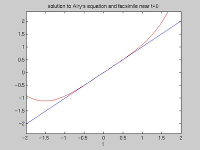
The facsimile agrees well with the actual solution in a neighborhood of the origin.
Solution for t near -16 = -4^2.
solb = ode45(airy, [0,-20], [0,1]);
tt = -18:.05:-14;
yy = deval(solb, tt, 1);
plot(tt, yy, 'r')
hold on
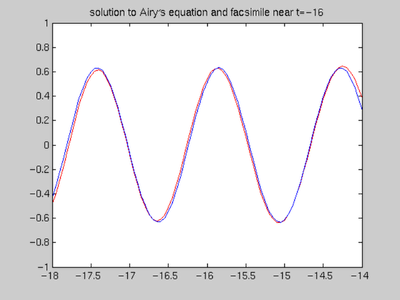
After viewing the graph, we see that it does resemble a sine curve. Now the solutions of y'' = -16*y are spanned by sin(4*t) and cos(4*t). So we want to find the best values of a(1) and a(2) for which yy ~ a(1)*sin(4*tt) + a(2)*cos(4*tt) We can do this with MATLAB's "backslash" command, as discussed in sections 4.1.3 and 8.4.
a = [sin(4*tt) ; cos(4*tt)]' \ yy'
facB = a(1)*sin(4*tt) + a(2)*cos(4*tt);
plot(tt, facB, 'b')
hold off
axis([-18 -14 -1 1])
title(['solution to Airy\prime', ...
    's equation and facsimile near t=-16'])
a =

   -0.3360
    0.5358
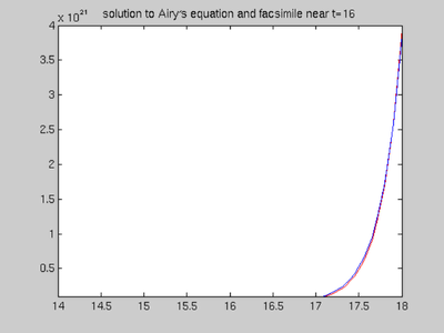
Solution for t near 16 = 4^2.
solf = ode45(airy, [0,18], [0,1]);
tt = 14:.05:18;
yy = deval(solf, tt, 1);
plot(tt, yy, 'r')
hold on
axis([14 18 10^20 4*10^21])
After viewing the graph, we see that it does resemble a hyperbolic sine curve. Now the solutions of y'' = -16*y are spanned by sinh(4*t) and cosh(4*t). So we want to find the best values of a(1) and a(2) for which yy ~ a(1)*sinh(4*tt) + a(2)*cosh(4*tt) We can do this with MATLAB's "backslash" command, as discussed in sections 4.1.3 and 8.4.
a = [sinh(4*tt) ; cosh(4*tt)]' \ yy'
facC = a(1)*sinh(4*tt) + a(2)*cosh(4*tt);
plot(tt, facC, 'b')
hold off
axis([14 18 10^20 4*10^21])
title(['solution to Airy\prime', ...
    's equation and facsimile near t=16'])
Warning: Rank deficient, rank = 1,  tol =    2.9111e+17.

a =

   1.0e-09 *

    0.4160
         0
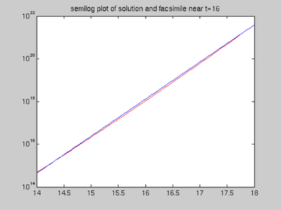
Since the solution is so large, we can get a better picture with a semilogarithmic plot. Recall that a semilog plot of an exponential function looks almost like a straight line.
semilogy(tt, yy, 'r', tt, facC, 'b')
title('semilog plot of solution and facsimile near t=16')

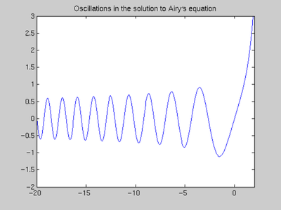
Solution over (-20,2), oscillations for negative time
ttb = -20:0.05:0;
yyb = deval(solb, ttb, 1);
ttf = 0:0.05:2;
yyf = deval(solf, ttf, 1);
plot(ttb, yyb, 'b', ttf, yyf, 'b')
axis([-20 2 -2 3])
title(['Oscillations in the solution to Airy\prime', ...
    's equation'])

It appears that the frequency increases and the amplitude decreases as t goes to minus infinity. The increasing frequency is predicted by our analysis; the decreasing amplitude is harder to explain.