See also: Generating Gaussian Random Fields.
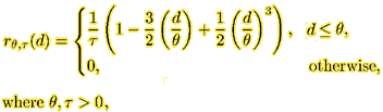
The covariance function r is defined as function(x, y, theta1, theta2, tau). For example, for the Spherical covariance function
|
sphercov <- function (x, y, theta1, theta2, tau) { d <- sqrt (x^2 + y^2) ifelse (d < theta1, (1- 1.5*(d/theta1)+0.5*(d/theta1)^3) / tau, 0) } |
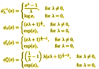
The transformation function, its inverse, and its two derivatives are defined as function(x, lambda). For example, for the Box-Cox model,
|
phiInv <- function (x, lambda) if (lambda==0) log(x) else (x^lambda-1)/lambda phi <- function(x, lambda) if (lambda==0) exp(x) else (x*lambda+1)^(1/lambda) phiPrime <- function (x, lambda) if (lambda==0) exp(x) else (x*lambda+1)^(1/lambda-1) phiDouble <- function (x, lambda) if (lambda==0) exp(x) else lambda * (1/lambda - 1) * (lambda * x + 1)^(1/lambda-2) |
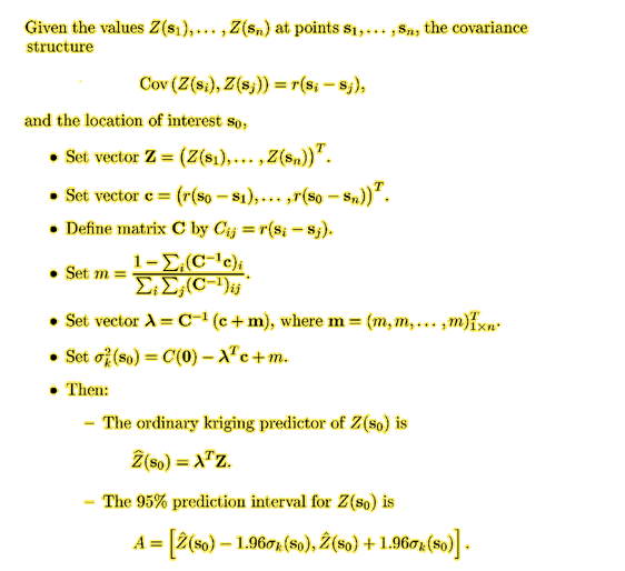
To perform kriging, the observed data must stored in the form of an n x 3 matrix, where each row represents an (x, y, z) point.
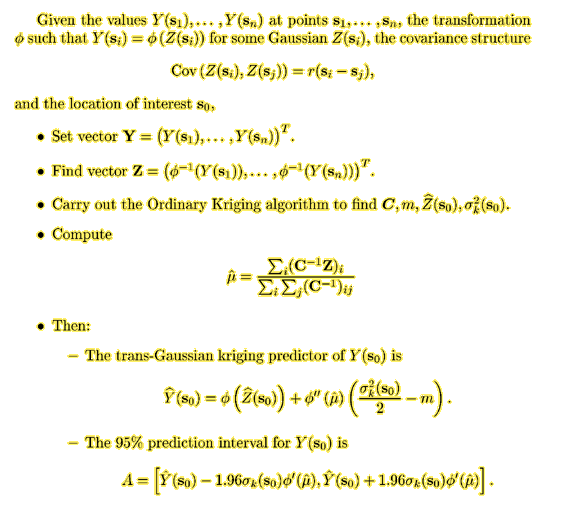
Then, the following function performs the trans-Gaussian kriging. The x- and y-coordinates of the locations at which the prediction is requested are passed to the function in the parameters sx and sy respectively.
|
kriging <- function(sx, sy, data, covfun, theta1,
theta2, tau, lambda=1) {
if (length(dim(data)) != 2 | dim(data)[2] != 3) stop("\nData must be an Nx3 matrix!") lensx <- length (sx) if (length(sy) != lensx) stop("\nsx and sy must be same length!") n <- dim(data)[1] x <- c(data[,rep(1:2, n)]) y <- c(t(data[,c(rep(1,n), rep(2,n))])) dif <- matrix(t(matrix(x - y, ncol=2*n)), ncol=2, byrow=T) C <- matrix (covfun(dif[,1], dif[,2], theta1, theta2, tau), nrow=n) Cinv <- solve(C) sumCinv <- sum(Cinv) Z <- c(phiInv(data[,3], lambda)) mu <- sum (Cinv %*% Z)/sumCinv prediction <- numeric(lensx) leftend <- numeric(lensx) rightend <- numeric(lensx) for (i in 1:lensx) { vectorc <- covfun(data[,1]-sx[i], data[,2]-sy[i], theta1, theta2, tau) m <- (1 - sum (Cinv %*% vectorc)) / sumCinv vectorlambda <- c((vectorc + m) %*% Cinv) sigma2 <- covfun(0, 0, theta1, theta2, tau) - sum(vectorlambda*vectorc) + m prediction[i] <- phi(sum(vectorlambda*Z), lambda) + phiDouble(mu, lambda) * (sigma2/2 - m) leftend[i] <- prediction[i] - 1.96*phiPrime(mu, lambda)*sqrt (sigma2) rightend[i] <- prediction[i] + 1.96*phiPrime(mu, lambda)*sqrt (sigma2) } list (prediction=prediction, leftend=leftend, rightend=rightend) } |
Suppose that you have a text file with x, y, z data. For example, run our on-line field generation script (another window will open), and "Save As" the file under the grey-level picture on the left into the directory from which you started Splus, under a name field.txt.
To perform the ordinary kriging prediction at location (4, 6) assuming a Spherical(4, 1, 1) covariance model, type
|
data <- matrix(scan(file="field.txt", skip=1),
byrow=T, ncol=3) kriging(4, 6, data, sphercov, 4, 1, 1) |
The trans-Gaussian kriging under the Box-Cox model requires positive data. We can shift the observations up by 10, and perform the trans-Gaussian kriging with lambda=0.5:
|
data[,3] <- data[,3] + 10 kriging(4, 6, data, sphercov, 4, 1, 1, 0.5) |
Start by enumerating the projections of the grid on the X and Y axis, for example
|
x <- seq (from=0, to=5, by=0.5) y <- seq (from=0, to=3, by=0.5) |
Now create a grid as the cartesian product of x and y by typing
|
grid <- cbind(c(matrix (rep (y, length(x)), ncol=length(y),
byrow=T)), rep (x, length(y))) |
To predict on the grid and save the point predictors to a variable called surface, type
|
surface <- kriging (grid[,1], grid[,2],
data, sphercov, 4, 1, 1)$prediction |
To view the prediction surface, type
| persp (x, y, matrix(surface, ncol=length(y))) |
To compare the prediction to the original (observed) surface, type
| persp (matrix(data[,3], ncol=4)) |
| write (t(cbind(grid, surface)), file = "pred3.txt", ncolumns=3) |
If you want to output Z values only, type
| write (t(surface), file = "predZ.txt") |