MATLAB Demo on 7.7-7.8: Differential Equations

Contents

Direction Fields

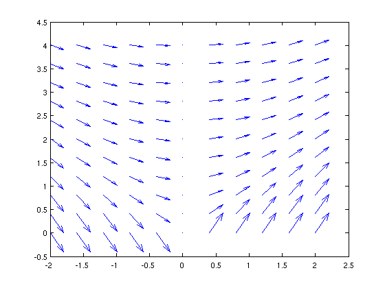
Let's start with a differential equation, say

At each point in the (x,y) plane (at least if y is not zero), this specifies what the slope of any solution curve must be. We can plot these to get a visual impression of the equation.

[xx, yy] = meshgrid(-2:.4:2,0.01:.4:4.01);
quiver(xx,yy,xx./xx,2*tanh(.5*xx./yy))

Solutions

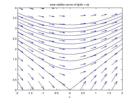
We can solve for the ``general solution'' of the equation.

syms x y
gensol=dsolve('Dy=x/y','x')
yfun = @(x, C1) eval(vectorize(gensol(1)))
hold on
for c=0:10
    ezplot(yfun(x,c),[-2,2]), axis([-2,2,0,4])
    title('some solution curves of dy/dx = x/y')
end
hold off

 
gensol =
 
  (x^2+C1)^(1/2)
 -(x^2+C1)^(1/2)
 
 

yfun = 

    @(x,C1)eval(vectorize(gensol(1)))

Another Example

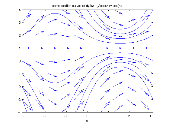
Let's look now at a linear equation,

Again we plot the direction field and some solution curves.

[xx, yy] = meshgrid(-pi:.2*pi:pi,-4:4);
quiver(xx,yy,xx./xx,2*tanh(.5*cos(xx).*(1-yy)))
lingensol=dsolve('Dy=(1-y)*cos(x)','x')
yfun2 = @(x, C1) eval(vectorize(lingensol))
hold on
for c=-4:4
    ezplot(yfun2(x,c),[-pi,pi]), axis([-pi,pi,-4,4])
    title('some solution curves of dy/dx + y*cos(x) = cos(x)')
end
hold off

 
lingensol =
 
1+exp(-sin(x))*C1
 
 

yfun2 = 

    @(x,C1)eval(vectorize(lingensol))

Published with MATLAB® 7.4