Calculus with MATLAB

Functions and Symbolic Differentiation
Problem 1:
Graphics and Plotting.
Problem 2:
Solving Equations
Problem 3:
Symbolic and Numerical Integration
Problem 4:
Additional Problems

In this published M-file we will try to present some of the central ideas involved in doing calculus with MATLAB. The central concept is that of a function. We will discuss first the representation of functions and then the ways of accomplishing the things we want to do with them. These fall into three broad categories: symbolic computation, numerical computation, and plotting, and we will deal with each of them in turn. We will try to provide concrete illustrations of each of the concepts involved as we go along. For the present, we will confine ourselves to functions of one variable. Later, we will need to discuss MATLAB's routines for dealing with functions of several variables.

Functions and Symbolic Differentiation

There are two distinct but related notions of function that are important in Calculus. One is a symbolic expression such as sin(x) or x^2. The other is a rule (algorithm) for producing a numerical output from a given numerical input or set of numerical inputs. This definition is more general; for example, it allows us to define a function f(x) to be x^2 in case x is negative or 0, and sin(x) in case x is positive. On the other hand, any symbolic expression implies a rule for evaluation. That is, if we know that f(x) = x^2, we know that f(4) = 4^2 = 16. In MATLAB, the fundamental difference between a function and a symbolic expression is that a function can be called with arguments and a symbolic expression cannot. However, a symbolic expression can be differentiated symbolically, while a function cannot. MATLAB functions can be created in three ways:

as anonymous functions or function handles (we learned about these in the last lesson, though without discussing what is "anonymous" about them, which is the fact that they can be used without naming them),
as function M-files, and
as inline functions (not especially recommended).

A typical way to define a symbolic expression is as follows:

syms x
f = x^2 - sin(x)

 
f =
 
x^2 - sin(x)

The next lines will show that we can differentiate f, but we cannot evaluate it, at least in the obvious way, since f(4) will give an error message (try it!). Notice that MATLAB recognizes what the "variable" is. In the case of several symbolic variables, we can specify the one with respect to which we want to differentiate.

diff(f)

 
ans =
 
2*x - cos(x)

We can evaluate f(4) by substituting 4 for x, or in other words, by typing

subs(f,x,4)

ans =

   16.7568

There are a few ways to convert f to a function. One is to define

fanon = @(t) subs(f, x, t)
fanon(4)

fanon = 

    @(t)subs(f,x,t)


ans =

   16.7568

What is going on here is that the x in f gets replaced by whatever the argument to the function is.

We can also turn f into an inline function with the command:

fin=inline(char(f))

fin =

     Inline function:
     fin(x) = x^2 - sin(x)

What's going on here is that the inline command requires a string as an input, and char turns f from a symbolic expression to the string 'x^2-sin(x)'. (If we had simply typed fin=inline(f) we'd get an error message, since f is not a string.) The inline function fin now accepts an argument:

fin(4)

ans =

   16.7568

Finally, there is another possible syntax:

ff = @(x) eval(vectorize(f))

ff = 

    @(x)eval(vectorize(f))

What's going on here is that vectorize is like char, though it is more flexible in that it will produce a string that can take a vector input. Then eval evaluates the resulting string. The result is a function that will operate on a vector input, as follows:

ff([0,pi])

ans =

         0    9.8696

Similarly we can construct a function, either inline or anonymous, from the derivative of f:

fxin=inline(char(diff(f)))

fxin =

     Inline function:
     fxin(x) = 2*x - cos(x)

Here the matlab function char replaces its argument by the string that represents it, thereby making it available to functions such as inline that demand strings as input.

Alternatively, we can try:

fxanon = @(t) subs(diff(f), x, t)
fxanon(4)

fxanon = 

    @(t)subs(diff(f),x,t)


ans =

    8.6536

The other way to create a function that can be evaluated is to write a function M-file. This is the primary way to define a function in most applications of MATLAB, although we shall be using it relatively seldom. The M-file can be created with the edit command, and you can print out its contents with the type command.

type fun1

function out=fun1(x)
out=x^2-sin(x);

fun1(4)

ans =

   16.7568

Problem 1:

Let

$$g(x) = x(e^x - x - 1).$$

a) Enter the formula for g(x) as a symbolic expression.
b) Obtain and name a symbolic expression for g'(x).
c) Evaluate g(4) and g'(4), using subs.
d) Evaluate g(4) and g'(4), by creating anonymous functions.
e) Evaluate g(4) by creating an M-file.

Graphics and Plotting.

One of the things we might want to do with a function is plot its graph. MATLAB's most elementary operation is to plot a point with specified coordinates.

plot(4,4)

The output from this command is the faint blue dot in the center of the figure. The way MATLAB plots a curve is to plot a sequence of dots connected by line segments. The input for such a plot consists of two vectors (lists of numbers). The first argument is the vector of x-coordinates and the second is the vector of y-coordinates. MATLAB connects dots whose coordinates appear in consecutive positions in the input vectors. Let us plot the function we defined in the previous section. First we prepare a vector of x-coordinates:

X1=-2:.5:2

X1 =

  Columns 1 through 7

   -2.0000   -1.5000   -1.0000   -0.5000         0    0.5000    1.0000

  Columns 8 through 9

    1.5000    2.0000

X1 is now a vector of nine components, starting with -2 and proceeding by increments of .5 to 2. Generally speaking, any command such as the one above creating a long vector should be terminated by a semicolon, to suppress the annoying written output.

We must now prepare an input vector of y-coordinates by applying our function to the x-coordinates. Our function fin will accomplish this, provided that "vectorize" it, i.e., we redefine it to be able to operate on vectors.

The matlab function vectorize replaces , ^, and / by ., .^, and ./ respectively. The significance of this is that MATLAB works primarily with vectors and matrices, and its default interpretation of multiplication, division, and exponentiation is as matrix operations. The dot before the operation indicates that it is to be performed entry by entry, even on matrices, which must therefore be the same shape. There is no difference between the dotted and undotted operations for numbers. However vectorized expressions are not interpreted as symbolic, in the sense that they cannot usually be symbolically differentiated. Fortunately, it is never necessary to do so.

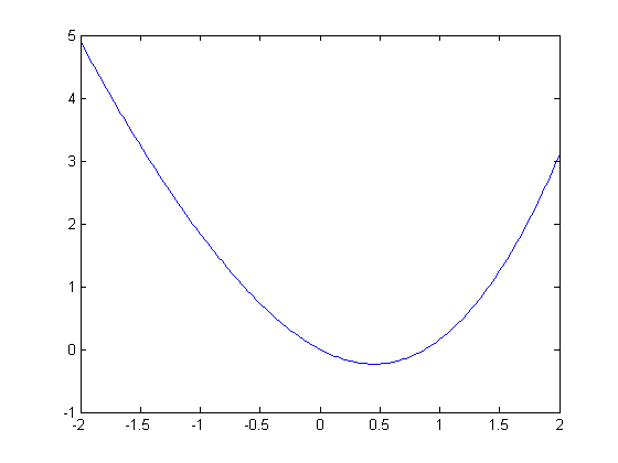
fin=inline(vectorize(f))
Y1=fin(X1)
plot(X1,Y1)

fin =

     Inline function:
     fin(x) = x.^2 - sin(x)


Y1 =

  Columns 1 through 7

    4.9093    3.2475    1.8415    0.7294         0   -0.2294    0.1585

  Columns 8 through 9

    1.2525    3.0907

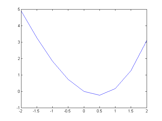
This plot is somewhat crude; we can see the corners. To remedy this we will decrease the step size. We will also insert semicolons after the definitions of X1 and Y1 to suppress the output.

X1=-2:.02:2;
Y1=fin(X1);
plot(X1,Y1)

Actually, the plotting of a symbolic function of one variable can be accomplished much more easily with the command ezplot, as in "Introduction to MATLAB". However, plot allows more direct control over the plotting process, and enables one to modify the color, appearance of the curves, etc. (Type doc plot for more on this.)

Problem 2:

Let the function g be as in Problem 1.

a) Plot g(x) for x between -3 and 3 using plot and a small enough step size to make the resulting curve reasonably smooth.
b) Plot g using ezplot.
c) Combine the previous plot with a plot of x^2 + 1. Plot enough of both curves so that you can be certain that the plot shows all points of intersection.

Solving Equations

The plot of f indicates that there are two solutions to the equation f(x) = 0, one of which is clearly 0. We have both solve, a symbolic equation solver, and fzero, a numerical equations solver, at our disposal. Let us illustrate solve first, but with an easier example.

g = x^2 - 7*x + 2
groots = solve(g)

 
g =
 
x^2 - 7*x + 2
 
 
groots =
 
 41^(1/2)/2 + 7/2
 7/2 - 41^(1/2)/2

Here solve finds all the roots it can, and reports them as the components of a column vector. Ordinarily, solve will solve for x, if present, or for the variable alphabetically closest to x otherwise. In the next example, y specifies the variable to solve for. Notice also that the first argument to solve is a symbolic expression, which solve sets equal to 0.

syms y
solve(x^2+y^2-4, y)

 
ans =
 
  (2 - x)^(1/2)*(x + 2)^(1/2)
 -(2 - x)^(1/2)*(x + 2)^(1/2)

Unfortunately, solve will not work very well on our function f, and may even cause MATLAB to hang. Let us try fzero instead, which solves equations numerically, using something akin to Newton's method, starting at a given initial value of the variable. The command fzero will not accept f as an argument, but it will accept the construct @fun1 (the @ is a marker for a function name) or an anonymous function.

newfroot=fzero(char(f),.8)
newfroot=fzero(fin,.8)
newfroot=fzero(@fun1,.8)

newfroot =

    0.8767


newfroot =

    0.8767


newfroot =

    0.8767

Problem 3:

Let g be as in Problems 1 and 2.

a) Referring to the plot in part c) of Problem 2, estimate those values of x for which g(x) = x^2 + 1.
b) Use solve to obtain more precise values and check the equation g(x) = x^2 + 1 for those values.

Symbolic and Numerical Integration

We have not yet dealt with integration. MATLAB has a symbolic integrator, called int, that will easily integrate f.

intsf=int(f,0,2)

 
intsf =
 
cos(2) + 5/3

However, if we replace f by the function h, defined buy

h=sqrt(x^2-sin(x^4))

 
h =
 
(x^2 - sin(x^4))^(1/2)

then int will be unable to evaluate the integral.

int(h,0,2)

Warning: Explicit integral could not be found. 
 
ans =
 
int((x^2 - sin(x^4))^(1/2), x = 0..2)

However, if we type double (standing for double-precision number) in front of the integral expression, MATLAB will return the result of a numerical integration.

double(int(h,0,2))

Warning: Explicit integral could not be found. 

ans =

    1.7196

We can check the plausibility of this answer by plotting h between 0 and 2 and estimating the area under the curve.

ezplot(h,[0,2])

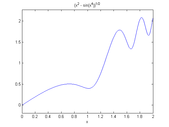
The numerical value returned by MATLAB is somewhat less than half the area of a square 2 units on a side. This appears to be consistent with our plot.

The numerical integration invoked by the combination of double and int is native, not to MATLAB, but to the symbolic engine MuPAD powering the Symbolic Math Toolbox. MATLAB also has its own numerical integrator called quadl. (The name comes from quadrature, an old word for numerical integration, and the "*l*" has something to do with the algorithm used, though there's no need for us to discuss it here.) The routines double(int(?)) and quadl(?) give slightly different answers, though usually they agree to several decimal places.

quadl(@(x) eval(vectorize(h)),0,2)

ans =

    1.7196

Problem 4:

Let g be as in previous problems.

a) Evaluate

$\int_{0}^3 g(x)\,dx$

symbolically, using int, and numerically using quadl. Compare your answers.

b) Evaluate

$\int_0^3 \sqrt{1 + (g'(x))^2}\,dx,$

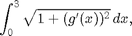
both using int and double, and using quadl.

c) Check the plausibility of your answers to part b) by means of an appropriate plot.

Additional Problems

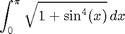
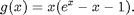
1. Let

$$f(x) = x^5 + 3x^4 - 3x + 7.$$

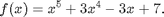
a) Plot f between x = -1 and x = 1.
b) Compute the derivative of f.
c) Use solve to find all critical points of f.
d) Find the extreme values of f on the interval [-1,1]. Hint: solve will store the critical points in a vector, which you cannot use unless you name it. Remember that you also need the values of f at 1 and -1.

2. Find all real roots of the equation x = 4 sin(x). You will need to use fzero.

3. Evaluate each of the following integrals, using both int and quadl.

$\int_0^\pi \sqrt{1 + \sin^2(x)}\,dx$

$\int_0^\pi \sqrt{1 + \sin^4(x)}\,dx$