Critical Points of Functions of Two and Three Variables
copyright © 2009 by Jonathan Rosenberg based on an earlier M-book, copyright © 2000 by Paul Green and Jonathan Rosenberg
Contents
Finding and Classifying Critical Points
We recall that a critical point of a function of several variables is a point at which the gradient of the function is either the zero vector 0 or is undefined. Although every point at which a function takes a local extreme value is a critical point, the converse is not true, just as in the single variable case. In this lesson we will be interested in identifying critical points of a function and classifying them. As in the single variable case, since the first partial derivatives vanish at every critical point, the classification depends on the values of the second partial derivatives. Let us illustrate what is involved with a specific example, namely the function defined below, which we have been considering throughout the past several notebooks.
syms x y z
f=((x^2-1)+(y^2-4)+(x^2-1)*(y^2-4))/(x^2+y^2+1)^2
f =

((x^2 - 1)*(y^2 - 4) + x^2 + y^2 - 5)/(x^2 + y^2 + 1)^2
To find the critical points of f we must set both partial derivatives of f to 0 and solve for x and y. We begin by computing the first partial derivatives of f.
fx=diff(f,x)
fy=diff(f,y)
fx =

(2*x + 2*x*(y^2 - 4))/(x^2 + y^2 + 1)^2 - (4*x*((x^2 - 1)*(y^2 - 4) + x^2 + y^2 - 5))/(x^2 + y^2 + 1)^3


fy =

(2*y + 2*y*(x^2 - 1))/(x^2 + y^2 + 1)^2 - (4*y*((x^2 - 1)*(y^2 - 4) + x^2 + y^2 - 5))/(x^2 + y^2 + 1)^3
To find critical points of f, we must set the partial derivatives equal to 0 and solve for x and y. Since the equations in this case are algebraic, we can use solve. (For more complicated functions built in part out of transcendental functions like exp, log, trig functions, etc., it may be be necessary to solve for the critical points numerically. More about this later.)
[xcr,ycr]=solve(fx,fy)
xcr =

              0
      3^(1/2)/3
     -3^(1/2)/3
  (2^(1/2)*i)/2
 -(2^(1/2)*i)/2
  (2^(1/2)*i)/2
 -(2^(1/2)*i)/2


ycr =

           0
           0
           0
  10^(1/2)/2
  10^(1/2)/2
 -10^(1/2)/2
 -10^(1/2)/2
Incidentally, it is worth pointing out a trick here. By default, the outputs xcr and ycr of the solve command are column vectors. As we have just typed the solve command, the vectors appear one after another. But a better alternative is:
[xcr,ycr]=solve(fx,fy); [xcr,ycr]
ans =

[              0,           0]
[      3^(1/2)/3,           0]
[     -3^(1/2)/3,           0]
[  (2^(1/2)*i)/2,  10^(1/2)/2]
[ -(2^(1/2)*i)/2,  10^(1/2)/2]
[  (2^(1/2)*i)/2, -10^(1/2)/2]
[ -(2^(1/2)*i)/2, -10^(1/2)/2]
Now xcr and ycr are stacked together in a matrix, so we can see each x-value together with the corresponding y-value. MATLAB has found seven critical points, of which the last four are not real. We now compute the second derivatives of f.
fxx=diff(fx,x)
fxy=diff(fx,y)
fyy=diff(fy,y)
fxx =

(2*y^2 - 6)/(x^2 + y^2 + 1)^2 - (4*((x^2 - 1)*(y^2 - 4) + x^2 + y^2 - 5))/(x^2 + y^2 + 1)^3 + (24*x^2*((x^2 - 1)*(y^2 - 4) + x^2 + y^2 - 5))/(x^2 + y^2 + 1)^4 - (8*x*(2*x + 2*x*(y^2 - 4)))/(x^2 + y^2 + 1)^3


fxy =

(4*x*y)/(x^2 + y^2 + 1)^2 - (4*y*(2*x + 2*x*(y^2 - 4)))/(x^2 + y^2 + 1)^3 - (4*x*(2*y + 2*y*(x^2 - 1)))/(x^2 + y^2 + 1)^3 + (24*x*y*((x^2 - 1)*(y^2 - 4) + x^2 + y^2 - 5))/(x^2 + y^2 + 1)^4


fyy =

(2*x^2)/(x^2 + y^2 + 1)^2 - (4*((x^2 - 1)*(y^2 - 4) + x^2 + y^2 - 5))/(x^2 + y^2 + 1)^3 + (24*y^2*((x^2 - 1)*(y^2 - 4) + x^2 + y^2 - 5))/(x^2 + y^2 + 1)^4 - (8*y*(2*y + 2*y*(x^2 - 1)))/(x^2 + y^2 + 1)^3
Of course there is no need to compute fyx, since for reasonable functions it always coincides with fxy. We compute the Hessian determinant (called the discriminant in your text) of the second partial derivatives, fxx*fyy-fxy^2, which is essential for the classification, and evaluate it at the critical points.
hessdetf=fxx*fyy-fxy^2
hessdetf =

((2*y^2 - 6)/(x^2 + y^2 + 1)^2 - (4*((x^2 - 1)*(y^2 - 4) + x^2 + y^2 - 5))/(x^2 + y^2 + 1)^3 + (24*x^2*((x^2 - 1)*(y^2 - 4) + x^2 + y^2 - 5))/(x^2 + y^2 + 1)^4 - (8*x*(2*x + 2*x*(y^2 - 4)))/(x^2 + y^2 + 1)^3)*((2*x^2)/(x^2 + y^2 + 1)^2 - (4*((x^2 - 1)*(y^2 - 4) + x^2 + y^2 - 5))/(x^2 + y^2 + 1)^3 + (24*y^2*((x^2 - 1)*(y^2 - 4) + x^2 + y^2 - 5))/(x^2 + y^2 + 1)^4 - (8*y*(2*y + 2*y*(x^2 - 1)))/(x^2 + y^2 + 1)^3) - (4*x*(2*y + 2*y*(x^2 - 1))/(x^2 + y^2 + 1)^3 + 4*y*(2*x + 2*x*(y^2 - 4))/(x^2 + y^2 + 1)^3 - 4*x*y/(x^2 + y^2 + 1)^2 - 24*x*y/(x^2 + y^2 + 1)^4*((x^2 - 1)*(y^2 - 4) + x^2 + y^2 - 5))^2
Another way to do the calculations, which is a little more elegant, is to use the jacobian command. Recall that this computes the gradient. But by using it twice, we can get the matrix of 2nd derivatives and then take the determinant.
gradf = jacobian(f, [x, y])
hessmatf = jacobian(gradf, [x, y])
hessdetf1 = simplify(det(hessmatf))
simplify(hessdetf - hessdetf1)
gradf =

[ (2*x + 2*x*(y^2 - 4))/(x^2 + y^2 + 1)^2 - (4*x*((x^2 - 1)*(y^2 - 4) + x^2 + y^2 - 5))/(x^2 + y^2 + 1)^3, (2*y + 2*y*(x^2 - 1))/(x^2 + y^2 + 1)^2 - (4*y*((x^2 - 1)*(y^2 - 4) + x^2 + y^2 - 5))/(x^2 + y^2 + 1)^3]


hessmatf =

[ (2*y^2 - 6)/(x^2 + y^2 + 1)^2 - (4*((x^2 - 1)*(y^2 - 4) + x^2 + y^2 - 5))/(x^2 + y^2 + 1)^3 + (24*x^2*((x^2 - 1)*(y^2 - 4) + x^2 + y^2 - 5))/(x^2 + y^2 + 1)^4 - (8*x*(2*x + 2*x*(y^2 - 4)))/(x^2 + y^2 + 1)^3,               (4*x*y)/(x^2 + y^2 + 1)^2 - (4*y*(2*x + 2*x*(y^2 - 4)))/(x^2 + y^2 + 1)^3 - (4*x*(2*y + 2*y*(x^2 - 1)))/(x^2 + y^2 + 1)^3 + (24*x*y*((x^2 - 1)*(y^2 - 4) + x^2 + y^2 - 5))/(x^2 + y^2 + 1)^4]
[                   (4*x*y)/(x^2 + y^2 + 1)^2 - (4*y*(2*x + 2*x*(y^2 - 4)))/(x^2 + y^2 + 1)^3 - (4*x*(2*y + 2*y*(x^2 - 1)))/(x^2 + y^2 + 1)^3 + (24*x*y*((x^2 - 1)*(y^2 - 4) + x^2 + y^2 - 5))/(x^2 + y^2 + 1)^4, (2*x^2)/(x^2 + y^2 + 1)^2 - (4*((x^2 - 1)*(y^2 - 4) + x^2 + y^2 - 5))/(x^2 + y^2 + 1)^3 + (24*y^2*((x^2 - 1)*(y^2 - 4) + x^2 + y^2 - 5))/(x^2 + y^2 + 1)^4 - (8*y*(2*y + 2*y*(x^2 - 1)))/(x^2 + y^2 + 1)^3]


hessdetf1 =

(x^6*(4*y^4 + 104*y^2 - 196) + x^4*(4*y^6 + 284*y^4 - 652*y^2 + 316) - x^2*(4*y^8 - 32*y^6 + 64*y^4 + 512*y^2 - 84) - x^8*(4*y^2 + 36) + 24*y^2 + 88*y^4 - 40*y^6 - 8)/(x^2 + y^2 + 1)^7


ans =

0
The fact that hessdetf - hessdetf1 simplified to 0 showed that both methods give the same thing.
The next step is to make a table of critical points, along with values of the Hessian determinant and the second partial derivative with respect to x. Since we are not interested in then non-real critical points, we can truncate the vectors xcr and ycr after the first three entries.
xcr = xcr(1:3); ycr = ycr(1:3);
for k = 1:3
    [xcr(k), ycr(k), subs(hessdetf, [x,y], [xcr(k), ycr(k)]), ...
       subs(fxx, [x,y], [xcr(k), ycr(k)])]
end
ans =

[ 0, 0, -8, -2]


ans =

[ 3^(1/2)/3, 0, 405/64, 27/16]


ans =

[ -3^(1/2)/3, 0, 405/64, 27/16]
Notice that all three of the real critical points are on the x-axis, and the first one is at the origin. Since the Hessian determinant is negative at the origin, we conclude that the critical point at the origin is a saddle point. The other two are local extrema and, since fxx is positive at both of them, they are local minima.
Let now reconstruct the contour and gradient plot we obtained for f in the last lesson.
[xx, yy] = meshgrid(-3:.1:3,-3:.1:3);
ffun = @(x,y) eval(vectorize(f));
fxfun = @(x,y) eval(vectorize(gradf(1)));
fyfun = @(x,y) eval(vectorize(gradf(2)));
contour(xx, yy, ffun(xx,yy), 30)
hold on
[xx, yy] = meshgrid(-3:.25:3,-3:.25:3);
quiver(xx, yy, fxfun(xx,yy), fyfun(xx,yy), 0.6)
axis equal tight, hold off
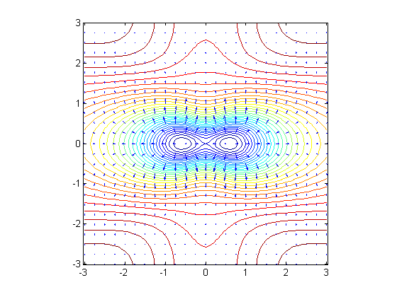
From the plot it is evident that there are two symmetrically placed local minima on the x-axis with a saddle point between them. We recognize the minima from the fact that they are surrounded by closed contours with the gradient arrows pointing outward. The pinching in of contours near the origin indicates a saddle point. The contour through the origin crosses itself, forming a transition between contours enclosing the two minima separately and contours enclosing them together.
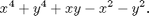
Problem 1:
Find and classify all critical points of the function
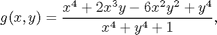
wich you studied in the previous lesson, and compare your results with the contour and gradient plot of g that you have already made.
Eigenvalues of the Hessian
We now take another look at the classification of critical points, with a view to extending it to functions of three or more variables. Let us define the function f2 and compute its first and second derivatives using MATLAB's symbolic jacobian operator.
f2=x^3-3*x^2+5*x*y-7*y^2
gradf2=jacobian(f2,[x,y])
hessmatf2=jacobian(gradf2,[x,y])
f2 =

x^3 - 3*x^2 + 5*x*y - 7*y^2


gradf2 =

[ 3*x^2 - 6*x + 5*y, 5*x - 14*y]


hessmatf2 =

[ 6*x - 6,   5]
[       5, -14]
The last output above is a symmetric matrix, known as the Hessian matrix, whose entries are the second partial derivatives of f. In order to find the critical points, we must again set the first partial derivatives equal to 0.
[xcr2,ycr2]=solve(gradf2(1),gradf2(2)); [xcr2,ycr2]
ans =

[     0,       0]
[ 59/42, 295/588]
There are two critical points. Let us now evaluate the Hessian matrix at the critical points.
H1=subs(hessmatf2,[x,y], [xcr2(1),ycr2(1)])
H2=subs(hessmatf2,[x,y], [xcr2(2),ycr2(2)])
H1 =

[ -6,   5]
[  5, -14]


H2 =

[ 17/7,   5]
[    5, -14]
At this point, however, instead of computing the Hessian determinant, which is the determinant of the Hessian matrix, we compute the eigenvalues of the matrix. The determinant of a matrix is the product of its eigenvalues, but the eigenvalues carry a lot more information than the determinant alone.
eig(H1)
eig(H2)
ans =

 - 41^(1/2) - 10
   41^(1/2) - 10


ans =

 - (25*29^(1/2))/14 - 81/14
   (25*29^(1/2))/14 - 81/14
We can obtain numerical versions with the double command:
double(eig(H1))
double(eig(H2))
ans =

  -16.4031
   -3.5969


ans =

  -15.4021
    3.8307
The significance of the eigenvalues of the Hessian matrix is that if all of them are positive at a critical point, the function has a local minimum there; if all are negative, the function has a local maximum; if they have mixed signs, the function has a saddle point; and if at least one of them is 0, the critical point is degenerate. These statements all generalize to functions of more than two variables, unlike the rule about the Hessian determinant. For functions of two variables, the determinant, being the product of the two eigenvalues, takes a negative value if and only if they have opposite signs. In the present case, we see that the critical point at the origin is a local maximum of f2, and the second critical point is a saddle point.
The point of this reformulation is that the Hessian matrix and its eigenvalues are just as easily computed and interpreted in the three-dimensional case. In this case, there will be three eigenvalues, all of which are positive at a local minimum and negative at a local maximum. A critical point of a function of three variables is degenerate if at least one of the eigenvalues of the Hessian matrix is 0, and has a saddle point in the remaining case, when at least one eigenvalue is positive, at least one is negative, and none is 0.
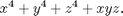
Problem 2:
Find and classify the critical points of the function

You may have trouble substituting the symbolic values of the coordinates of the critical points into the Hessian matrix; if so, convert them to numerical values, using double.
A Graphical/Numerical Method
For some functions (especially if they involve transcendental functions such as exp, log, sin, cos, etc.), the formulas for the partial derivatives may be too complicated to use solve to find the critical points. In this case, a graphical or numerical method may be necessary. Here is an example:
k=x*sin(y)+y^2*cos(x)
kx=diff(k,x)
ky=diff(k,y)
k =

y^2*cos(x) + x*sin(y)


kx =

sin(y) - y^2*sin(x)


ky =

x*cos(y) + 2*y*cos(x)
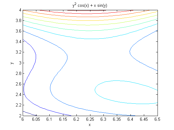
In this case solving analytically for the solutions of kx = 0, ky = 0 is going to be hopeless. Also, we can't solve numerically without knowing how many solutions there are and roughly where they are located. The way out is therefore to draw plots of the solutions to kx = 0 and to ky = 0. Then we see where these curves intersect and can use the graphical information to get starting values for the use of a numerical solver. In our particular example, we can try:
[x1,y1]=meshgrid(-8:.1:8,-8:.1:8);
kxfun=@(x,y) eval(vectorize(kx)); kyfun=@(x,y) eval(vectorize(ky));
contour(x1,y1,kxfun(x1,y1),[0,0],'r'), hold on
contour(x1,y1,kyfun(x1,y1),[0,0],'b'), hold off
Here the plot of kx = 0 is shown in red and the plot of ky = 0 is shown in blue. Thus, for example, we have critical points near (6.2, 2.4) and near (6.2, 3.2). We can locate them more accurately using the M-file newton2d.m, which uses a two-dimensional version of Newton's method to solve more accurately:
type newton2d.m
function [xsol, ysol] = newton2d(varargin)
%NEWTON2D 2-dimensional Newton's method
% The command
% [xsol, ysol] = newton2d(eq1, eq2, xstart, ystart)
% searches for a root of the simultaneous (nonlinear)
% equations eq1=0 and eq2=0, starting from the initial
% guesses x=xstart, y=ystart.  Here eq1 and eq2 should be
% entered as strings in the variables 'x' and 'y' or
% as symbolic expressions in x and y. Alternatively,
% [xsol, ysol] = newton2d(eq1, eq2, xvar, yvar, xstart, ystart)
% allows one to specify the names of the independent variables.
% The optional argument 'maxiterations' at the end specifies the
% maximum number of iterations to try. The default is 20.
%
% Example: [xsol, ysol] = newton2d('x^2 + y^2 - 4', 'x - y', 1, 1)
% gives the output
% xsol =
%
%    1.4142
%
%
% ysol =
%
%    1.4142
%
%
% written by Jonathan Rosenberg, 8/10/99
% revised 8/22/05

if nargin<4
    error('not enough input arguments -- need at least the two equations and starting values for x and y');
end

if nargin>7, error('too many input arguments'); end

eq1=varargin{1}; eq2=varargin{2};
if ischar(eq1) & ~ischar(eq2)
    error('both equations must be of same form: strings or symbolic')
end
if ~ischar(eq1) & ischar(eq2)
    error('both equations must be of same form: strings or symbolic')
end
% Default value of maxiterations is 20.
maxiterations=20;
% Default values of xvar and yvar are 'x', 'y'.
if nargin<6
    xvar = 'x'; yvar = 'y'; xstart = varargin{3}; ystart = varargin{4};
end
if nargin>5
    xvar = varargin{3}; yvar = varargin{4};
    xstart = varargin{5}; ystart = varargin{6};
end
if nargin==5, maxiterations=varargin{5}; end
if nargin==7, maxiterations=varargin{7}; end

% Start by computing partial derivatives.
f11 = diff(sym(eq1), xvar);
f12 = diff(sym(eq1), yvar);
f21 = diff(sym(eq2), xvar);
f22 = diff(sym(eq2), yvar);
% Vector functions for evaluation
F1  = inline(vectorize(eq1),xvar,yvar);
F2  = inline(vectorize(eq2),xvar,yvar);
A11 = inline(vectorize(f11),xvar,yvar);
A12 = inline(vectorize(f21),xvar,yvar);
A21 = inline(vectorize(f12),xvar,yvar);
A22 = inline(vectorize(f22),xvar,yvar);
X  = [xstart, ystart];
for counter=1:maxiterations
A  = [A11(X(1), X(2)), A12(X(1), X(2)); A21(X(1), X(2)), A22(X(1), X(2))];
F = [F1(X(1), X(2)), F2(X(1), X(2))];
    if max(abs(F)) < eps, xsol=X(1);
% process has converged
    ysol=X(2); return; end
    if condest(A) > 10^10, error('matrix of partial derivatives singular or almost singular -- try again with different starting values'); end
    X  = X - F/A;
end
xsol=X(1); ysol=X(2);
[xsol,ysol]=newton2d(kx, ky, 6.2, 2.4); [xsol,ysol]
[xsol,ysol]=newton2d(kx, ky, 6.2, 3.2); [xsol,ysol]
ans =

    6.3954    2.4237


ans =

    6.2832    3.1416
Thus we have critical points near (6.3954, 2.4237) and (6.2832, 3.1416). The second of these looks suspiciously like (2*pi, pi), and in fact we have
subs(kx, [x,y], sym('[2*pi,pi]'))
subs(ky, [x,y], sym('[2*pi,pi]'))
ans =

0


ans =

0
so this hunch is in fact correct. To classify these critical points, we can compute
hessdetk = simplify(diff(kx, x)*diff(ky, y) - diff(kx, y)^2)
double(subs(hessdetk, [x,y], [6.3954, 2.4237]))
double(subs(diff(kx, x), [x,y], [6.3954, 2.4237]))
double(subs(hessdetk, [x,y], [2*pi, pi]))
hessdetk =

- (cos(y) - 2*y*sin(x))^2 - y^2*cos(x)*(2*cos(x) - x*sin(y))


ans =

   11.2762


ans =

   -5.8374


ans =

  -20.7392
so the first point, (6.3954, 2.4237), has positive Hessian determinant, negative 2nd derivative with respect to x, and is thus a local maximum. Similarly the point (2*pi, pi) is a saddle point. One could also check these calculations with a contour plot:
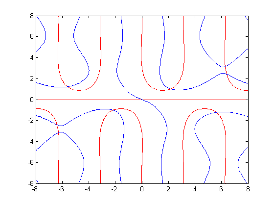
ezcontour(k, [6, 6.5, 2, 4])
The picture indeed shows contours looping around the local maximum at (6.3954, 2.4237) and the characteristic shape of a saddle near (6.2832, 3.1416).
Additional Problems:
- 1. Find and classify all critical points of the function
Relate your results to a simultaneous contour and gradient plot of the function.
- 2. Find and classify all critical points of the function
MATLAB will report many critical points, but only a few of them are real.
- 3. Find and classify all critical points of the function h(x, y) = y^2*exp(x^2) - x - 3*y. You will need the graphical/numerical method to find the critical points.
- 4. Find and classify all critical points of the function h(x, y) = y^2*exp(x) - x - 3*y. Use both the analytical and the graphical/numerical methods to find the critical points, and compare the results.