Space Curves, Frenet Frames, and Torsion
Copyright © 2000 by Paul Green and Jonathan Rosenberg
In this notebook, we will plot curves in 3-dimensional space and compute their invariants. As we proceed we will provide a detailed discussion of some mathematical concepts that are not mentioned in Ellis and Gulick. In order to have a concrete example before us, we consider the twisted cubic, parametrized by (t, t2 ,t3).
[ t, t^2, t^3]
It will be convenient to define MATLAB function m-files veclength.m and unitvec.m which return respectively the magnitude of a vector and the vector divided by its magnitude. The Frenet frame of a curve at a point is a triple of vectors (T, N, B) consisting of the unit tangent vector T at that point, the unit normal N (the unit vector in the direction of the derivative of the unit tangent), and the unit binormal B = T x N, the cross-product of the unit tangent with the unit normal. We calculate the Frenet frame for the twisted cubic:
[ 1, 2*t, 3*t^2]
tctan=simplify(unitvec(tcvel))
[ 1/(1+4*t^2+9*t^4)^(1/2), 2*t/(1+4*t^2+9*t^4)^(1/2), 3*t^2/(1+4*t^2+9*t^4)^(1/2)]
[ 0, 2, 6*t]
Because the acceleration a is not parallel to the unit normal N, but the cross-product v x a of the velocity and the acceleration is parallel to the unit binormal B, it is convenient to compute the unit binormal before the unit normal vector.
[ 6*t^2, -6*t, 2]
tcbin=simplify(unitvec(tccross))
[ 3*t^2/(9*t^4+9*t^2+1)^(1/2), -3*t/(9*t^4+9*t^2+1)^(1/2), 1/(9*t^4+9*t^2+1)^(1/2)]
Since T is perpendicular to N and B = T x N, the three unit vectors T, N, and B are mutually perpendicular, and it follows that also N = B x T and T = N x B. This gives the fastest way to compute N.
tcnorm=simplify(cross(tcbin,tctan))
[ -t*(2+9*t^2)/(9*t^4+9*t^2+1)^(1/2)/(1+4*t^2+9*t^4)^(1/2), -(-1+9*t^4)/(9*t^4+9*t^2+1)^(1/2)/(1+4*t^2+9*t^4)^(1/2), 3*t*(2*t^2+1)/(9*t^4+9*t^2+1)^(1/2)/(1+4*t^2+9*t^4)^(1/2)]
We recall that the curvature, while defined as the magnitude of the derivative of the unit tangent with respect to arclength, is most conveniently computed as follows:
tccurve=simplify(veclength(tccross)/veclength(tcvel)^3)
2*(9*t^4+9*t^2+1)^(1/2)/(1+4*t^2+9*t^4)^(3/2)
Problem 1:
Consider the trefoil parametrized by
trefoil=[(2+cos(3*t))*cos(2*t),(2+cos(3*t))*sin(2*t),cos(3*t)]
[ (2+cos(3*t))*cos(2*t), (2+cos(3*t))*sin(2*t), cos(3*t)]
(a) Plot the trefoil for t between 0 and 2p.
(b) Compute the curvature of the trefoil.
(c) Compute the Frenet frame of the trefoil.
We could also have defined the curvature as the normal
component of the derivative of the unit tangent with respect to arclength. The
two definitions are synonymous because the derivative of the unit tangent, either
with respect to the parameter t or with respect to arclength s,
is parallel to the unit normal. Symbolically, what we have so far, if ![]() denotes the curvature, is
denotes the curvature, is
![]()
![]()
![]()
![]() .
.
From this it follows since ![]() , that
, that
![]()
![]() ,
,
which explains the formula for the curvature.
We are now interested in the derivative of the unit normal
with respect to arclength. By differentiating the equation ![]() with respect to s,
we obtain
with respect to s,
we obtain ![]() , from which it follows that
, from which it follows that ![]() . Since N is a unit
vector, we know that
. Since N is a unit
vector, we know that ![]() is perpendicular to N. The torsion
is perpendicular to N. The torsion ![]() is defined to be
is defined to be ![]() . Note that since the direction of B is determined independently of
. Note that since the direction of B is determined independently of
![]() , the torsion, unlike the curvature, is signed. Notice also
that for a plane curve, the binormal is identically perpendicular to the plane
in which the curve lies and the torsion is 0.Thus we have the Frenet-Serret
formulae:
, the torsion, unlike the curvature, is signed. Notice also
that for a plane curve, the binormal is identically perpendicular to the plane
in which the curve lies and the torsion is 0.Thus we have the Frenet-Serret
formulae:
![]()
![]()
![]()
The last of these is easily obtained by differentiating the
equations ![]() and
and ![]() with respect to s.
Note that, since the direction of B is determined independently of
with respect to s.
Note that, since the direction of B is determined independently of ![]() , the torsion, unlike the curvature, is signed. Notice also
that for a plane curve, the binormal is identically perpendicular to the plane
in which the curve lies, and the torsion is 0.
, the torsion, unlike the curvature, is signed. Notice also
that for a plane curve, the binormal is identically perpendicular to the plane
in which the curve lies, and the torsion is 0.
Next, we compute ![]() . We begin by
differentiating the equation
. We begin by
differentiating the equation
![]()
which we established earlier. The product and chain rules will generate many terms , but the only one that is not perpendicular to B is the one that comes from differentiating N. Thus we have
![]()
Multiplying both sides by the coefficient of ![]() , and using the
identity,
, and using the
identity, ![]()
![]() , we obtain
, we obtain

which yields a convenient formula for the torsion. In the case of the twisted cubic, it gives
[ 0, 0, 6]
tctors=simplify(realdot(tccross,tcthird)/realdot(tccross,tccross))
3/(9*t^4+9*t^2+1)
Problem 2:
Compute the torsion of the trefoil.
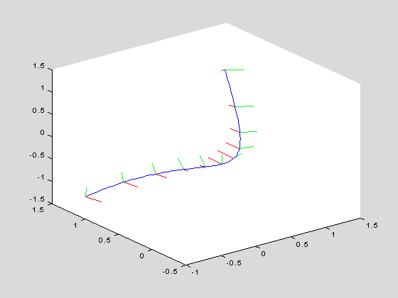
To begin to see the geometrical significance of the torsion, we use the m-file curveframeplot.m. This plots the curve in blue together with normal vectors in red and binormal vectors in green. The tangent vectors are not plotted since the tangent direction is clear from the curve. The last two arguments determine the number of frames plotted and the length of the normal and binormal vectors.
curveframeplot(twistcube,'t',-1,1,10,.2)
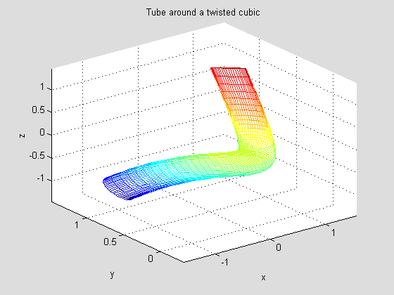
Notice how the Frenet frames twist around the curve as the parameter changes. To make this even clearer, we define and plot a tube around the curve. We will need a second parameter since the tube is a surface.
tctube=twistcube+ .2*cos(s)*tcnorm+.2*sin(s)*tcbin
[ t-1/5*cos(s)*t*(2+9*t^2)/(9*t^4+9*t^2+1)^(1/2)/(1+4*t^2+9*t^4)^(1/2)+3/5*sin(s)*t^2/(9*t^4+9*t^2+1)^(1/2), t^2-1/5*cos(s)*(-1+9*t^4)/(9*t^4+9*t^2+1)^(1/2)/(1+4*t^2+9*t^4)^(1/2)-3/5*sin(s)*t/(9*t^4+9*t^2+1)^(1/2), t^3+3/5*cos(s)*t*(2*t^2+1)/(9*t^4+9*t^2+1)^(1/2)/(1+4*t^2+9*t^4)^(1/2)+1/5*sin(s)/(9*t^4+9*t^2+1)^(1/2)]
In this case, the input is more illuminating than the output. For fixed t, s parametrizes a circle around the tube. For fixed s, t parametrizes a curve running along the tube and, in the presence of torsion, twisting around it. We will plot the tube using ezmesh. The first three arguments are the components of tctube; the last argument gives the limits for s and t in the form [smin, smax, tmin, tmax]:
ezmesh(tctube(1),tctube(2),tctube(3),[0,2*pi,-1,1])
title('Tube around a twisted cubic')
The torsion is illustrated by the way in which the longitudinal mesh lines, corresponding to constant values of s, twist around the tube.
Problem 3:
(a) Use curveframeplot to plot the trefoil with its Frenet frame.
(b) Use ezsurf to show the twisting of the Frenet frame of the trefoil around the curve.
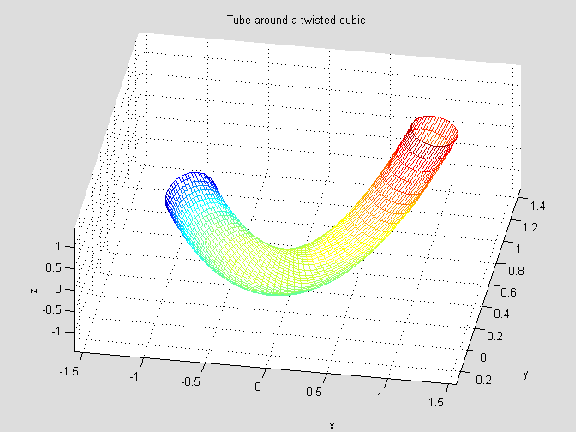
We will take this opportunity to illustrate how the graphical capabilities of MATLAB can be used more fully. When a plot command is executed, the default notebook option embeds the graphic in the notebook as a Picture file. If we either turn off the embedding option, or execute the command directly in the MATLAB command window, the graphic is created in a MATLAB figure window, where it can be manipulated in many ways and saved as a fig file. The fig file can then be embedded back in the notebook, using the 'open' command.
In this case, we have reexecuted the ezsurf command in the MATLAB command window, then used the capabilities of the MATLAB figure window to rotate the picture, saved the result as 'tubeplot.fig', and opened it in the notebook below.
title('Tube around a twisted cubic')
Additional Problems
1. Consider the family of helices parametrized by (R cos(t), R sin(t), A t).
(a) Compute the torsion and curvature as functions of R and A.
(b) For R=A=1, plot the helix, showing the Frenet frame at several points along the curve.
(c) Plot the tube of radius .2 around the helix showing the twisting of the Frenet frame around the helix.
2. Consider the curve parametrized by (t-2t2, t2+t3, t+2t3-2).
(a) Compute the torsion and the binormal.
(b) What do you deduce about the curve from the result of part a)?
(c) Provide a graphical demonstration of your conclusion in part b).


