Evaluating Triple Integrals
copyright © 2009 by Jonathan Rosenberg based on an earlier M-book, copyright © 2000 by Paul Green and Jonathan Rosenberg
Contents
Evaluating Triple Iterated Integrals
In passing from double to triple integrals, there is much less that is novel than in passing from single to double integrals. MATLAB has a built-in triple integrator triplequad similar to dblquad, but again, it only integrates over rectangular boxes. However, more general threefold iterated integrals can be formulated and evaluated using the symbolic toolbox's routines, in the same manner as twofold iterated integrals. And if the first of the three integrals can be evaluated symbolically, it is then possible to use dblquad for the remaining integrations.
Example 1
We will begin by considering the iterated integral
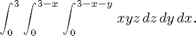
We can evaluate this easily as
syms x y z
firstans=int(int(int(x*y*z,z,0,3-x-y),y,0,3-x),x,0,3)
firstans =

81/80
We can also evaluate the first integral only, and then use dblquad or numint2 for the remaining two integrations:
f=int(x*y*z,z,0,3-x-y)
secondans=numint2(f,y,0,3-x,x,0,3)
f =

(x*y*(x + y - 3)^2)/2


secondans =

    1.0125
Let's see how the answers compare:
double(firstans-secondans)
ans =

     0
To use triplequad here, we would again have to make a change of variables


So in the new coordinates, the integral is over the box 0<x<3, 0<u<1, 0<v<1 and the integrand is


and the integral can be computed as
h = @(x,u,v) x.*(3-x).^4.*u.*(1-u).^2.*v;
thirdans = triplequad(h, 0, 3, 0, 1, 0, 1)
thirdans =

    1.0125
with accuracy
double(firstans-thirdans)
ans =

     0
But because dblquad is sometimes slow (and the same algorithm extrapolated to three dimensions would be even slower) or doesn't work very well, we have looked for an alternative, based on a freeware package of M-files called the numerical integration toolbox. This toolbox is much faster and more adaptable (though admittedly sometimes harder to use) than dblquad. Copy this package from http://www.math.umd.edu/users/jmr/241/mfiles/nit/ into a subdirectory of your working directory called nit. To use this package, first add the package with the command:
addpath nit
To see how it works, we first try out an alternative version of numint2, based on nit, called newnumint2. The syntax is the same as for numint2, but there is an optional final parameter, which is the number of subdivision points to use in each direction. (The default is 20.) The higher this parameter, the more accurate the results; however, the running time of the algorithm is proportional to the square of this parameter, so be careful about increasing it.
fourthans=newnumint2(f,y,0,3-x,x,0,3)
fourthans =

    1.0125
Note that this answer looks the same as the first two to four decimal places, but that we are spared all the annoying warning messages. The accuracy is:
double(firstans-fourthans)
ans =

     0
which is pretty good!! Now we try a totally numerical integration. The analogue of newnumint2 for triple integrals is called numint3. Again there is an optional final parameter, which is the number of subdivision points to use in each direction. (The default is 8.) The higher this parameter, the more accurate the results; however, the running time of the algorithm is proportional to the cube of this parameter, so be extra careful about increasing it.
fourthans=numint3(x*y*z,z,0,3-x-y,y,0,3-x,x,0,3)
fourthans =

    1.0125
The accuracy is:
double(firstans-fourthans)
ans =

     0
Again pretty good!
Problem 1
Evaluate the threefold iterated integral
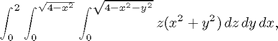
both symbolically and numerically. (For the numerical integration, first do the integral over z, then use newnumint2 on this intermediate result.)
Finding the Limits
The remaining issue in the evaluation of triple integrals is the determination of limits. Once this has been done, the actual integration can always be performed by one of the methods illustrated above.
Example 2
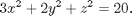
Let us consider the region above the paraboloid

and inside the ellipsoid
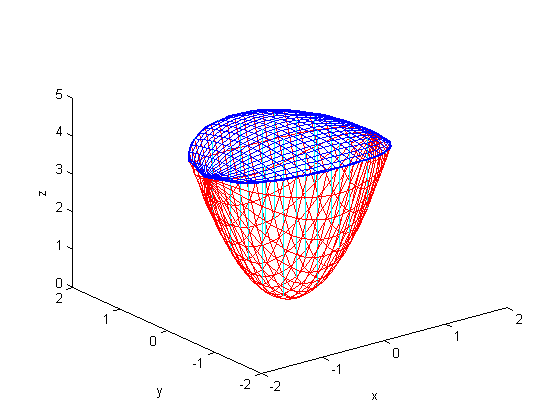
We might begin by plotting the two surfaces simultaneously. Since z is never negative on or above the paraboloid, we are interested only in positive values of z. Consequently, we will solve the equation of the ellipsoid for positive z and use ezmesh to plot both surfaces.
ezmesh(sqrt(20-3*x^2-2*y^2),[-3,3,-2,2]);
hold on
ezmesh(2*x^2+3*y^2, [-3,3,-2,2])
view([1,2,3])
hold off;
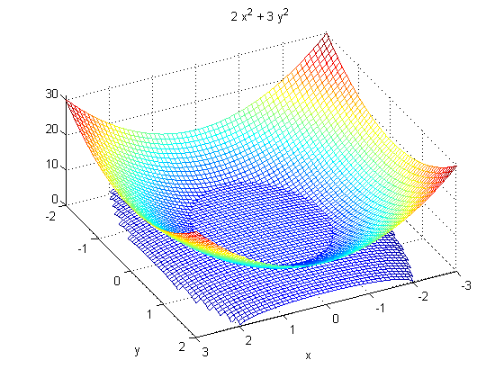
From the viewpoint we have chosen, using MATLAB's view comand, we can see that there is a region inside the ellipsoid that is bounded below by the paraboloid and above by the ellipsoid. This determines the lower and upper limits for z. Accordingly, we set
z1=2*x^2 + 3*y^2
z2=sqrt(20-3*x^2-2*y^2)
z1 =

2*x^2 + 3*y^2


z2 =

(20 - 2*y^2 - 3*x^2)^(1/2)
To determine the limits for x and y, it may be helpful to plot the curve along which the upper and lower limits for z coincide. We will do this using ezplot:
ezplot(z2-z1, [-3, 3, -2, 2])
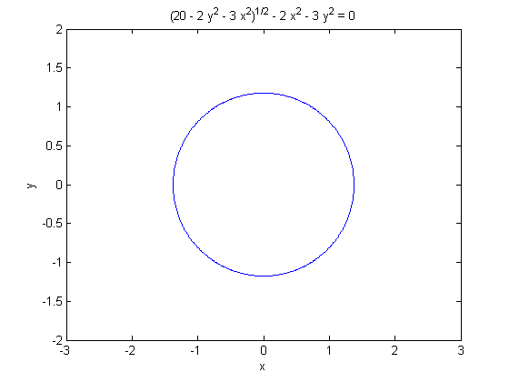
Although this looks like an ellipse, it is actually a quartic curve. We will establish the limits by solving the equation of the curve for y as a function of x. We expect two solutions, corresponding to the upper and lower y limits, and we should be able to determine the x limits by setting the y limits equal to each other.
ylims=solve(z2-z1,y)
ylims =

    ((4*(181 - 15*x^2)^(1/2))/9 - (8*x^2)/3 - 4/9)^(1/2)/2
  (- (8*x^2)/3 - (4*(181 - 15*x^2)^(1/2))/9 - 4/9)^(1/2)/2
   -((4*(181 - 15*x^2)^(1/2))/9 - (8*x^2)/3 - 4/9)^(1/2)/2
 -(- (8*x^2)/3 - (4*(181 - 15*x^2)^(1/2))/9 - 4/9)^(1/2)/2
Here solve has found four solutions instead of two. This should not surprise us too much since the equation in question is quartic. Of the four solutions, however, two of them are complex, as we can see by substituting x=0.
double(subs(ylims,x,0))
ans =

   1.1763
   0.0000 + 1.2673i
  -1.1763
  -0.0000 - 1.2673i
Thus solution #3 should be the lower limit for y, solution #1 should be the upper limit, and solutions #2 and 4 are complex and should be discarded. So we set
y1=ylims(3)
y2=ylims(1)
xlims=solve(y2-y1,x)
x1=double(xlims(2))
x2=double(xlims(1))
y1 =

-((4*(181 - 15*x^2)^(1/2))/9 - (8*x^2)/3 - 4/9)^(1/2)/2


y2 =

((4*(181 - 15*x^2)^(1/2))/9 - (8*x^2)/3 - 4/9)^(1/2)/2


xlims =

  (329^(1/2)/2 - 3/2)^(1/2)/2
 -(329^(1/2)/2 - 3/2)^(1/2)/2


x1 =

   -1.3756


x2 =

    1.3756
We can now check our limits for geometric plausibility. For this purpose we have written an M-file called viewSolid.
type viewSolid
function viewSolid(zvar, F, G, yvar, f, g, xvar, a, b)
%VIEWSOLID is a version for MATLAB of the routine on page 161
%  of "Multivariable Calculus and Mathematica" for viewing the region
%  bounded by two surfaces for the purpose of setting up triple integrals.
%  The arguments are entered from the inside out.
%  There are two forms of the command --- either f, g,
%  F, and G can be vectorized functions, or else they can
%  be symbolic expressions. xvar, yvar, and zvar can be
%  either symbolic variables or strings.
%  The variable xvar (x, for example) is on the
%  OUTSIDE of the triple integral, and goes between CONSTANT limits a and b.
%  The variable yvar goes in the MIDDLE of the triple integral, and goes
%  between limits which must be expressions in one variable [xvar].
%  The variable zvar goes in the INSIDE of the triple integral, and goes
%  between limits which must be expressions in two
%  variables [xvar and yvar].  The lower surface is plotted in red, the
%  upper one in blue, and the "hatching" in cyan.
%
% Examples: viewSolid(z, 0, (x+y)/4, y, x/2, x, x, 1, 2)
% gives the picture on page 163 of "Multivariable Calculus and Mathematica"
% and the picture on page 164 of "Multivariable Calculus and Mathematica"
% can be produced by
%     viewSolid(z, x^2+3*y^2, 4-y^2, y, -sqrt(4-x^2)/2, sqrt(4-x^2)/2, ...
%               x, -2, 2,)
% One can also type viewSolid('z', @(x,y) 0, ...
% @(x,y)(x+y)/4, 'y', @(x) x/2, @(x) x, 'x', 1, 2)
%

if isa(f, 'sym') % case of symbolic input
    ffun=inline(vectorize(f+0*xvar),char(xvar));
    gfun=inline(vectorize(g+0*xvar),char(xvar));
    Ffun=inline(vectorize(F+0*xvar),char(xvar),char(yvar));
    Gfun=inline(vectorize(G+0*xvar),char(xvar),char(yvar));
    oldviewSolid(char(xvar), double(a), double(b), ...
       char(yvar), ffun, gfun, char(zvar), Ffun, Gfun)
else
   oldviewSolid(char(xvar), double(a), double(b), ...
       char(yvar), f, g, char(zvar), F, G)
end
%%%%%%% subfunction goes here %%%%%%
function oldviewSolid(xvar, a, b, yvar, f, g, zvar, F, G)
for counter=0:20
  xx = a + (counter/20)*(b-a);
  YY = f(xx)*ones(1, 21)+((g(xx)-f(xx))/20)*(0:20);
  XX = xx*ones(1, 21);
%% The next lines inserted to make bounding curves thicker.
  widthpar=0.5;
  if counter==0, widthpar=2; end
  if counter==20, widthpar=2; end
%% Plot curves of constant x on surface patches.
 plot3(XX, YY, F(XX, YY).*ones(1,21), 'r', 'LineWidth', widthpar);
 hold on
 plot3(XX, YY, G(XX, YY).*ones(1,21), 'b', 'LineWidth', widthpar);
end;
%% Now do the same thing in the other direction.
XX = a*ones(1, 21)+((b-a)/20)*(0:20);
%% Normalize sizes of vectors.
YY=0:2; ZZ1=0:20; ZZ2=0:20;
for counter=0:20,
%% The next lines inserted to make bounding curves thicker.
  widthpar=0.5;
  if counter==0, widthpar=2; end
  if counter==20, widthpar=2; end
    for i=1:21,
       YY(i)=f(XX(i))+(counter/20)*(g(XX(i))-f(XX(i)));
       ZZ1(i)=F(XX(i),YY(i));
       ZZ2(i)=G(XX(i),YY(i));
    end;
  plot3(XX, YY, ZZ1, 'r', 'LineWidth',widthpar);
  plot3(XX, YY, ZZ2, 'b', 'LineWidth',widthpar);
end;
%% Now plot vertical lines.
for u = 0:0.2:1,
  for v = 0:0.2:1,
   x=a + (b-a)*u; y = f(a + (b-a)*u) +(g(a + (b-a)*u)-f(a + (b-a)*u))*v;
   plot3([x, x], [y, y], [F(x,y), G(x, y)], 'c');
  end;
end;
xlabel(xvar)
ylabel(yvar)
zlabel(zvar)
hold off
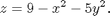
It takes a proposed set of limits of integration (written from the inside to the outside) and draws a picture of the corresponding region.
viewSolid(z,z1,z2,y,y1,y2,x,x1,x2)
This looks reasonable; we may now use the limits we have found to integrate any function we like over the region in question.
Problem 2
Find the appropriate limits for integrating over the region bounded by the paraboloids

and
Check your results using viewSolid.
What is special about the examples we have just considered is that the region in question is bounded by two surfaces, each of which has an equation specifying z as a function of x and y. The procedure we have used in this case will work for any such region, as long as solve is able to solve the associated equations. We will look now at an example of another sort.
Example 3
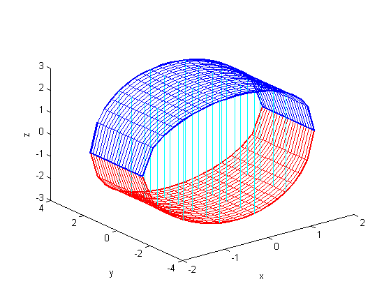
We consider the region interior to both of the elliptical cylinders, x^2+2y^2 = 9 and 2x^2+z^2 = 8. We begin by observing that the condition that a point be interior to both cylinders constrains x^2 to be at most 4. We also observe that, for fixed x, the limits for y and z are determined independently of each other. So we'll want to put the x-integral on the outside. We can immediately set
x1=-2; x2=2;
y1=-sqrt((9-x^2)/2); y2=-y1;
z1=-sqrt(8-2*x^2); z2=-z1;
We can again use viewSolid to check the plausibility of these limits, although the resulting plot is more difficult to interpret in this case, since it shows only the upper and lower boundaries as surfaces; the side boundaries are shown as ensembles of vertical lines.
viewSolid(z,z1,z2,y,y1,y2,x,x1,x2)
Problem 3
Find limits appropriate for integrating over the solid region bounded by the paraboloid y = x^2 + z^2 - 2 and the cylinder x^2 + y^2 = 1. Check your results with viewSolid.
Additional Problems:
1. Find the volume of each of the solid regions considered in Examples 2 and 3 and Problems 2 and 3 above. Use at least two different methods in each case and compare the answers.
2. Integrate the function x^2 + y*z over the solid region above the paraboloid z = x^2 + y^2 and below the plane x + y + z = 10.
3. Integrate the function x^2 + 2y^2 + 3z^2 over the solid region interior to both the sphere x^2 + y^2 + z^2 = 9 and the cylinder (x-1)^2 + y^2 = 1.