Stochastic differential equations (SDEs) have become an important modeling tool in numerous areas of science and engineering. For example, molecular motion, gene expression, ecosystems, stock price evolution, mechanical systems and many others are often modeled using SDEs. Often the phenomena of interest such as conformal changes in molecules, genetic switches, financial crises, failure of a mechanical system occur rarely on the timescale of the system which makes their prediction and analysis by direnct simulation infeasible. My research is devoted to the development of deterministic numerical methods for quantification of such rare events. The theoretical fundation for these methods is Freidlin's and Wetzell's large deviation theory.
The quasipotential is a key concept of Freidlin's and Wentzell's large deviation theory for SDEs with small white noise. If the SDE is gradient, i.e.,
dx = - ∇ V(x)dt + ε1/2dw,
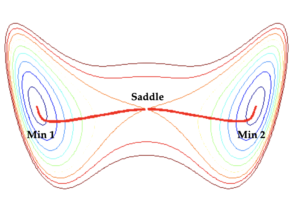
x ∈ Rn, the system spends most of the time near minima of the potential function V(x) (we assume that it is smooth and has a finite number of local minima one of which is the global minimum). The invariant probability measure is the Gibbs measure μ(x) = Z-1exp(-2V(x)/ε) . Moreover, let us assume that as ε tends to zero and that local minima xi and xj are separated by a saddle xij , and this is the saddle with the lowest value of V(x) lying on the boundary of the basin of attraction of xi. Then, with probability very close to one, transition from small neighborhood of xi to a small neignborhood of xj happens within a small tube surronding the path φ(t) going first directly uphill to the saddle xij, dφ/dt = ∇ V(φ), hen directly downhill to xj, dφ/dt = -∇V(φ). Furthermore, the expected exit time from the basin of xi is logarithmically equivalent to exp(2(V(xij) - V(xi))/ε) and the prefactor also can be found analytically.
If the SDEs is nongradient
dx = b(x)dt + ε1/2dw,
where b(x) is a smooth nongradient vector field with a finite number of isolated attractors, the situation is more complicated. To obtain estimates for the invariant probability measure, maximum likelihood transition paths, and expected exit times from basins of attractors, one needs to decompose b(x) to a potential component and orthogonal to it rotational component in each basin of attraction:b(x)= -(1/2)∇ U(x) + l(x),
∇ U(x) ⊥ l(x).
The potential component of this decomposition is called the quasi-potential. Unfortunately, this decomposition can be done analytically only in special cases. Hence, we develop numerical methods to compute this decomposition. We solve the following variational problem on a mesh:Once the quasipotential U(x) is computed with respect to an attractor A, the invariant probability measure in the basin B(A) scales as
μ(x) ≍ exp(-U(x)/ε),
the expected exit time from the basin of A scales asτA ≍ exp [ minx∈ ∂ B(A)U(x)/ε ],
and the maximum likelihood exit path φ followis the rotational component l(x) and goes agains the potential component:d φ/dt = l(φ) + (1/2)∇ U(φ).
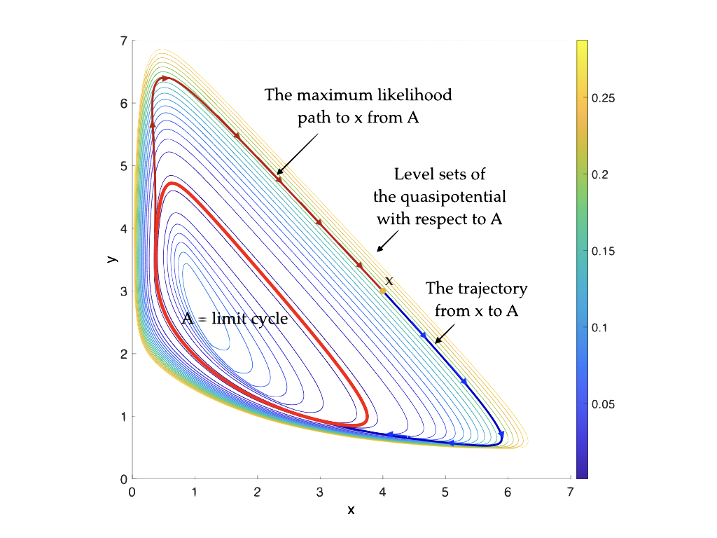 |
The computed quasipotential (level sets), a maximum likelihood path from the stable limit cycle to a point x, and a trajectory from x to the limit cycle for Brusselator |
Quasipotential solvers
- OUM 2D: A quasi-potential solver based on Sethian's and Vladimirski's ordered upwind method (Cameron, 2012)
- OUM 2D: An R-package QPot (Nolting, C. Moore, C. Stieha, M. Cameron, K. Abbott, 2016)
- OLIM 2D Ordered line integral methods (OLIMs) (Dahiya and Cameron, 2018). Software is available.
- OLIM 2D for SDEs with variable and anisotropic diffusion. (Dahiya and Cameron, 2018) Software is available.
- OLIM 3D The OLIM is rationalized and promoted to 3D. (Yang, Potter, Cameron, 2019) Software is available.
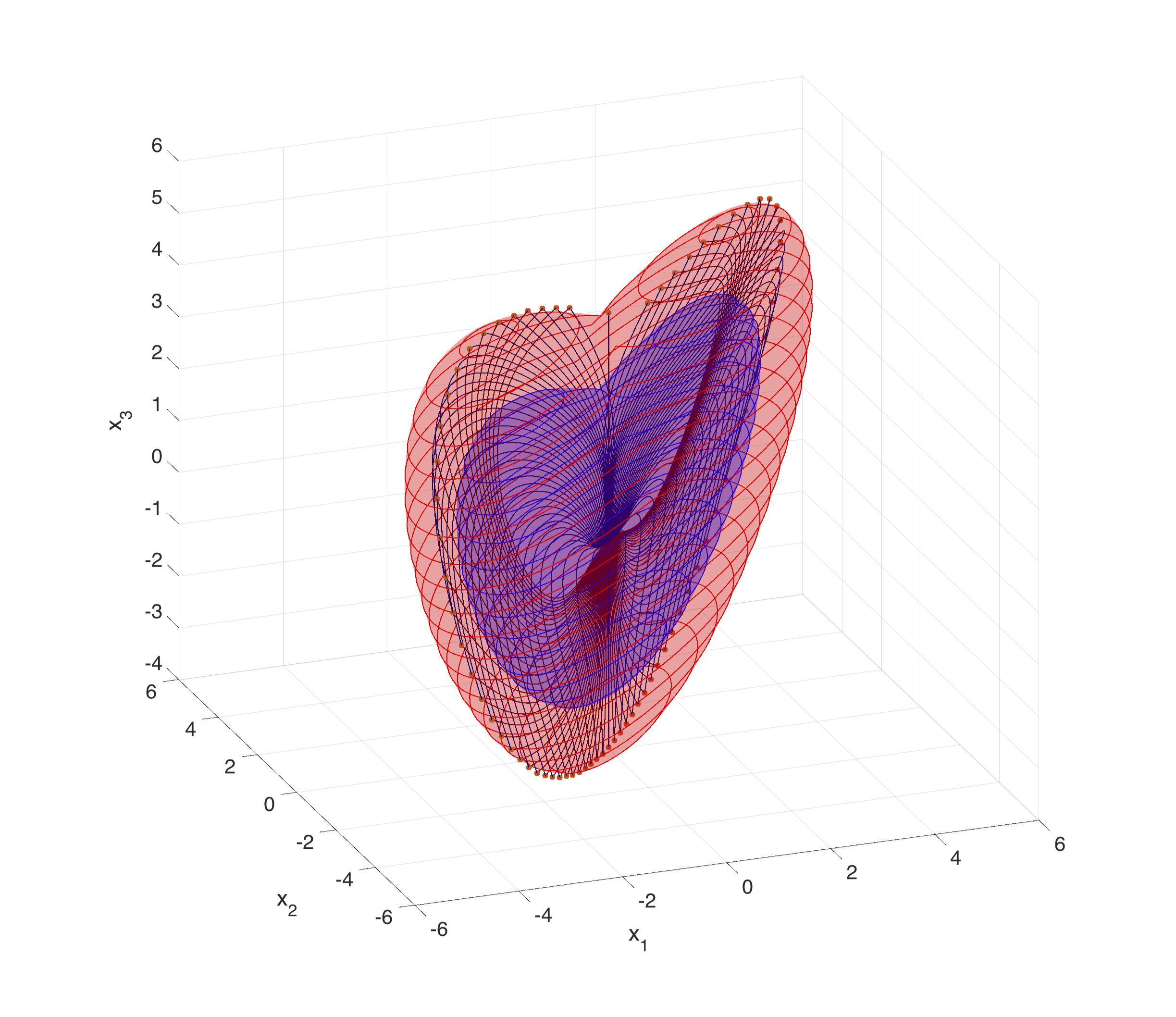
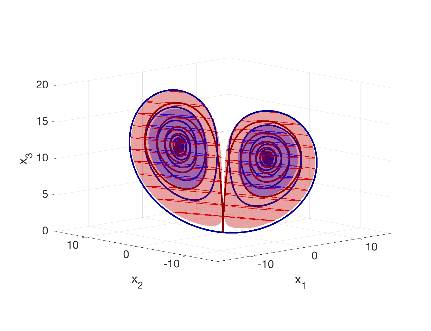
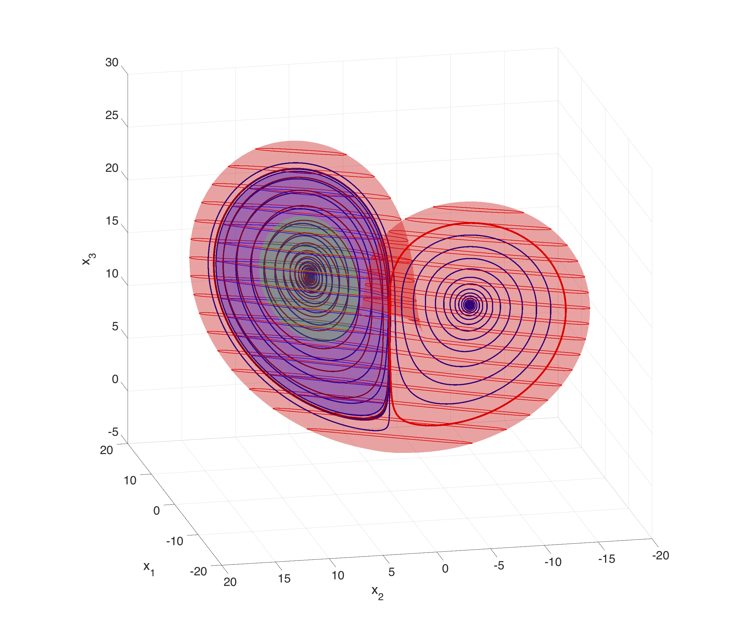
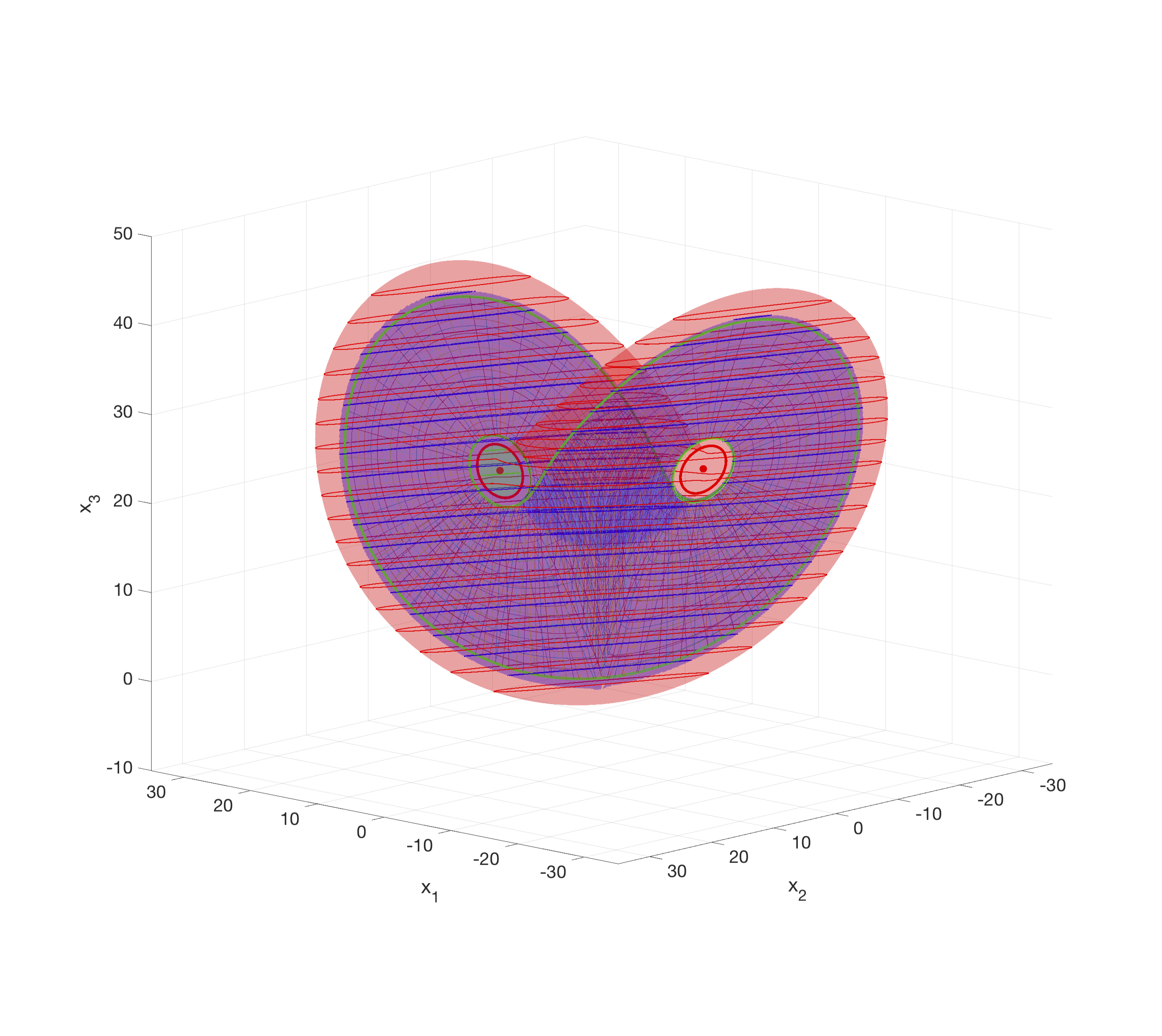
- Application to stochastic Lorenz'63 (Cameron and Yang, 2019) Software is available. Github: OLIM-for-Lorenz63
Stochastic Lorenz'63 (click on image to see a video)
- Level sets of the quasipotential,
- trajectories (fat dark blue curves),
- maximum likelihood transition paths (fat red curves),
 |
 |
 |
 |