Example for interpolation
Contents
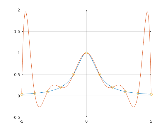
Interpolation with equidistant nodes
We want to approximate the function f(x) = 1/(1+x^2) on the interval [-5,5]
f = @(x) 1./(1+x.^2);          % define function f
a = -5; b = 5;                 % endpoints of interval
n = 11;                        % number of nodes for interpolation
xt = linspace(-5,5,1000);      % use these x values for plotting

xe = a + (0:n-1)*(b-a)/(n-1);  % equidistant nodes, same as  xe = linspace(a,b,n)
ye = f(xe);                    % find values of f at nodes xe

d = divdiff(xe,ye);            % use divided difference algorithm to find coefficients d

pt = evnewt(d,xe,xt);          % evaluate interpolating polynomial at points xt
plot(xt,f(xt),xt,pt,xe,ye,'o'); grid on  % plot function f and interpolating polynomial
                                         % mark given points with 'o'
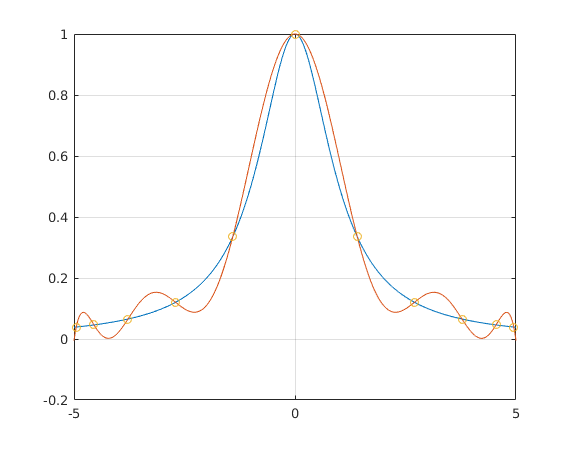
Interpolation with Chebyshev nodes
xc = (a+b)/2 + (b-a)/2*cos(pi/n*((1:n)-.5));      % Chebyshev nodes
yc = f(xc);                    % find values of f at nodes xc

d = divdiff(xc,yc);            % use divided difference algorithm to find coefficients d
pt = evnewt(d,xc,xt);          % evaluate interpolating polynomial at points xt

plot(xt,f(xt),xt,pt,xc,yc,'o'); grid on  % plot function f and interpolating polynomial
                                         % mark given points with 'o'
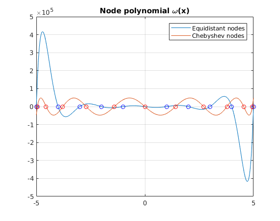
Compare node polynomials
We plot the node polynomial (x-x_1)...(x-x_n) for equidistant nodes and for Chebyshev nodes.
Note:
- The Chebyshev nodes have a wider spacing near the center, and are closer together near the endpoints of the interval [a,b]
- The node polynomial for equidistant nodes becomes huge near the endpoints
- The node polynomial for Chebyshev nodes has oscillations of uniform size
ye = ones(size(xt));           % equidistant nodes: evaluate (x-x_1)...(x-x_n) for xt values
for j=1:n
  ye = ye.*(xt-xe(j));
end

yc = ones(size(xt));           % Chebyshev nodes: evaluate (x-x_1)...(x-x_n) for xt values
for j=1:n
  yc = yc.*(xt-xc(j));
end

plot(xt,ye,xt,yc); hold on     % plot node polynomials
plot(xe,zeros(1,n),'bo',xc,zeros(1,n),'ro') ; hold off  % mark nodes with 'o'
grid on;
title('Node polynomial \omega(x)')
legend('Equidistant nodes','Chebyshev nodes')