Predator-Prey Problem
Contents
- Download this m-file
- System of differential equations
- Given initial conditions
- Definition of the function f
- Solve the ODE using the Euler method
- Solve the initial value problem using ode45
- Plot both y1(t) and y2(t) vs. t
- Plot y2 vs. y1 (phase plane plot)
- Solve ODE with higher accuracy, then make phase plane plot
Download this m-file
You first have to download the file
and put it in the same directory as your other m-files.
System of differential equations
Let y1 denote the number of rabbits (prey), let y2 denote the number of foxes (predator). The population growth is described by
- y1' = a1*y1
- y2' = a2*y2
Here the growth rate a1 for rabbits is positive for y2=0, but decreases with increasing y2; the growth rate a2 for foxes is negative for y1=0, but increases with increasing y1:
- a1 = 2 - .5*y2
- a2 = -1 + .5*y1
Hence we obtain the following system of ODEs
- y1' = (2-.5*y2)*y1
- y2' = (-1+.5*y1)*y2
Given initial conditions
The initial rabbit population is 6, the initial fox population is 2:
- y1(0) = 6
- y2(0) = 2
Definition of the function f
We have an ODE system y' = f(t,y) where y is a vector and the vector-valued function f is given by
f = @(t,y) [(2-.5*y(2))*y(1); (-1+.5*y(1))*y(2)];
Solve the ODE using the Euler method
Assume that at time t we have the vector y. Then we compute the slope vector s=f(t,y) and define the new y-vector by y = y + h*s.
We repeat this until we reach the final time T.
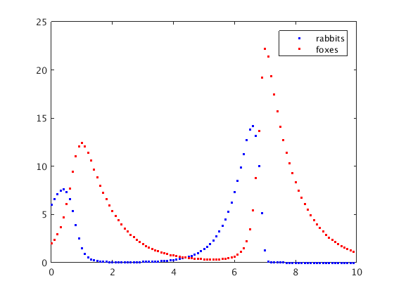
Note that the values of the Euler method are not very accurate for h=0.1.
y = [6;2]; t = 0;           % given initial value
h = .1;                     % step size

for i=1:100
  plot(t,y(1),'b.',t,y(2),'r.'); hold on    % plot rabbits in blue, foxes in red
  s = f(t,y);               % find slope vector
  y = y + h*s;              % find new y-vector by using s
  t = t + h;
end
hold off
legend('rabbits','foxes')
Solve the initial value problem using ode45
We want to find the functions y1(t) and y2(t) for t in [0,15].
In Matlab we use [ts,ys] = ode45(f,[t0,T],y0).
Here the input arguments are:
- f is the ODE function (can be defined by an @-function, or an m-file)
- t0 is the initial time
- T is the final time
- y0 is the initial y-vector at time t0.
This returns the arrays ts, ys:
- ts is the vector of time values (Matlab chooses h automatically at each step)
- ys is an array containing the values of y: row j contains the values of y1 (rabbits) and y2 (foxes) at the time ts(j) .
[ts,ys] gives a table with t in column 1, y1 (rabbits) in column 2, y2 (foxes) in column 3
[ts,ys] = ode45(f,[0,15],[6;2]);
[ts,ys]                          % table with values of t, y1, y2 in each row
ans =
         0    6.0000    2.0000
    0.0251    6.1486    2.1050
    0.0502    6.2923    2.2196
    0.0754    6.4296    2.3446
    0.1005    6.5591    2.4808
    0.2069    6.9969    3.1941
    0.3133    7.1111    4.1963
    0.4197    6.7843    5.4927
    0.5262    6.0208    6.9653
    0.6137    5.1515    8.1505
    0.7013    4.1971    9.1635
    0.7888    3.2782    9.9004
    0.8763    2.4945   10.3010
    0.9560    1.9375   10.3842
    1.0357    1.5046   10.2662
    1.1153    1.1755    9.9993
    1.1950    0.9308    9.6282
    1.3057    0.6956    9.0121
    1.4163    0.5356    8.3476
    1.5270    0.4187    7.6803
    1.6377    0.3389    7.0278
    1.7386    0.2951    6.4553
    1.8395    0.2644    5.9184
    1.9404    0.2430    5.4190
    2.0413    0.2288    4.9575
    2.1513    0.2199    4.4964
    2.2612    0.2165    4.0768
    2.3711    0.2179    3.6961
    2.4811    0.2237    3.3517
    2.6374    0.2395    2.9189
    2.7937    0.2645    2.5460
    2.9499    0.3002    2.2261
    3.1062    0.3487    1.9527
    3.3371    0.4508    1.6229
    3.5679    0.6020    1.3683
    3.7988    0.8248    1.1784
    4.0296    1.1519    1.0472
    4.1967    1.4775    0.9889
    4.3638    1.9031    0.9627
    4.5309    2.4532    0.9754
    4.6980    3.1507    1.0418
    4.8650    4.0046    1.1925
    5.0321    5.0184    1.4699
    5.1992    6.0903    1.9739
    5.3663    6.9628    2.8857
    5.4157    7.1245    3.2691
    5.4652    7.2152    3.7155
    5.5146    7.2210    4.2281
    5.5640    7.1303    4.8061
    5.6135    6.9355    5.4442
    5.6629    6.6364    6.1291
    5.7124    6.2414    6.8408
    5.7618    5.7669    7.5537
    5.8406    4.9091    8.6141
    5.9193    4.0192    9.4919
    5.9981    3.1857   10.1190
    6.0769    2.4763   10.4609
    6.1518    1.9408   10.5379
    6.2268    1.5209   10.4293
    6.3017    1.1983   10.1813
    6.3767    0.9553    9.8339
    6.4820    0.7155    9.2451
    6.5873    0.5508    8.6030
    6.6926    0.4307    7.9520
    6.7980    0.3479    7.3110
    6.8961    0.3000    6.7334
    6.9942    0.2660    6.1891
    7.0924    0.2419    5.6807
    7.1905    0.2252    5.2090
    7.2970    0.2139    4.7376
    7.4035    0.2081    4.3069
    7.5101    0.2069    3.9147
    7.6166    0.2098    3.5584
    7.7638    0.2204    3.1202
    7.9110    0.2385    2.7388
    8.0582    0.2650    2.4080
    8.2054    0.3012    2.1220
    8.4423    0.3854    1.7435
    8.6792    0.5125    1.4502
    8.9161    0.7027    1.2285
    9.1530    0.9859    1.0699
    9.3284    1.2790    0.9914
    9.5038    1.6692    0.9458
    9.6791    2.1839    0.9381
    9.8545    2.8522    0.9805
    9.9937    3.5072    1.0657
   10.1329    4.2840    1.2148
   10.2721    5.1624    1.4650
   10.4112    6.0746    1.8844
   10.5057    6.6519    2.3133
   10.6002    7.1044    2.9173
   10.6947    7.3348    3.7426
   10.7892    7.2474    4.8119
   10.8574    6.9411    5.7304
   10.9256    6.4349    6.7267
   10.9938    5.7649    7.7362
   11.0620    4.9923    8.6823
   11.1302    4.1965    9.4829
   11.1984    3.4424   10.0883
   11.2666    2.7736   10.4783
   11.3348    2.2138   10.6557
   11.4057    1.7487   10.6446
   11.4766    1.3848   10.4801
   11.5475    1.1036   10.2026
   11.6184    0.8899    9.8454
   11.7113    0.6877    9.3046
   11.8041    0.5445    8.7247
   11.8970    0.4397    8.1366
   11.9899    0.3646    7.5568
   12.0920    0.3089    6.9412
   12.1941    0.2699    6.3603
   12.2962    0.2425    5.8184
   12.3983    0.2237    5.3165
   12.5019    0.2116    4.8476
   12.6055    0.2048    4.4178
   12.7090    0.2025    4.0252
   12.8126    0.2041    3.6675
   12.9561    0.2125    3.2250
   13.0996    0.2278    2.8383
   13.2430    0.2507    2.5014
   13.3865    0.2823    2.2088
   13.6312    0.3609    1.7983
   13.8759    0.4819    1.4818
   14.1207    0.6659    1.2432
   14.3654    0.9441    1.0725
   14.5240    1.1946    0.9959
   14.6827    1.5195    0.9458
   14.8413    1.9384    0.9247
   15.0000    2.4731    0.9392
Plot both y1(t) and y2(t) vs. t
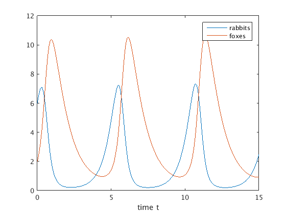
We can plot the rabbit population vs. t using plot(ts,ys(:,1)) since ys(:,1) gives the first column of the array ys with the rabbit values.
We can plot both rabbits and foxes vs. t using plot(ts,ys). Matlab now plots the first column of ys (rabbits) in blue, and the second column of ys (foxes) in red.
It appears that the functions y1(t), y2(t) are periodic with a period of about 5.
plot(ts,ys)              % plot rabbit and fox population vs. t
legend('rabbits','foxes'); xlabel('time t')
Plot y2 vs. y1 (phase plane plot)
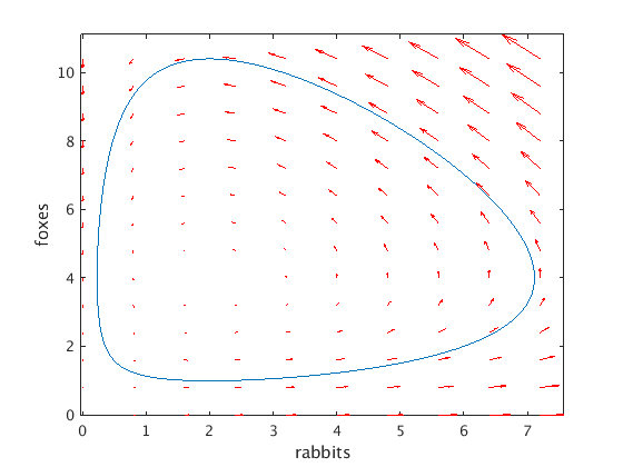
We can also consider the solution (y1(t),y2(t)) as tracing a curve in the (y1,y2) plane ("phase plane"). We can plot this curve with plot(ys(:,1),ys(:,2)).
The phase plane plot should be a closed curve since the solution is periodic.
The vector field given by f shows the velocity vectors with which the point (y1(t),y2(t)) moves along the trajectory. We see that the point moves along the closed curve counterclockwise as t increases.
Note that we do not quite get a closed curve: after one period we arrive at a slightly different point. This is due to the error of the numerical method in ode45.
plot(ys(:,1),ys(:,2)); hold on               % plot solution in phase plane
xlabel('rabbits'); ylabel('foxes')
vectfield(f,0:.8:7.5,0:.8:10.5); hold off    % plot vector field
Solve ODE with higher accuracy, then make phase plane plot
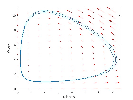
We can define additional options using odeset. Here we specify a tolerance of 1e-10 for both the relative error ('RelTol') and the absolute error ('AbsTol').
Now the errors are much smaller, and we obtain a closed curve (at least for the visual accuracy of the plot).
opt = odeset('RelTol',1e-10,'AbsTol',1e-10);  % use smaller tolerances
[ts,ys] = ode45(f,[0,15],[6;2],opt);          % use opt defined by odeset
plot(ys(:,1),ys(:,2)); hold on                % plot solution in phase plane
xlabel('rabbits'); ylabel('foxes')
vectfield(f,0:.8:7.5,0:.8:10.5); hold off     % plot vector field