Interpolate a periodic function by trigonometric polynomial, even number of nodes
Contents
Plot function and interpolation points
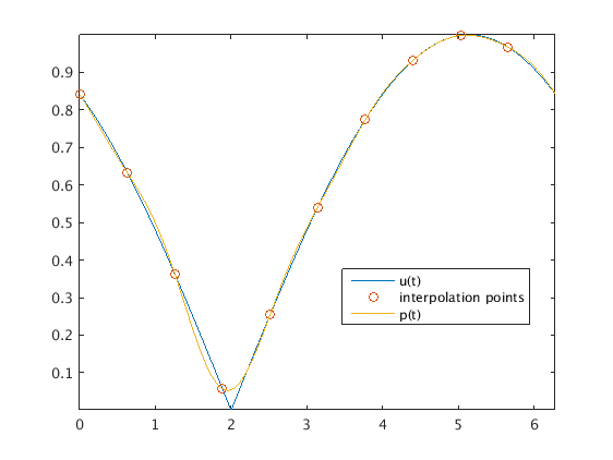
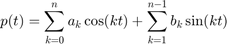
We want to approximate the 2 pi periodic function u(t) = abs(sin(t/2-1)) using  with n=5. This space has dimension m=10, so we use 10 equidistant data points j*2*pi/m, j=0,...,m-1.
u = @(t) abs(sin(t/2-1));
m = 10;                    % even number of data points
t = (0:m-1)'*2*pi/m;       % interpolation points

U = u(t);                  % data used for interpolation

mp = 1000;                 % for plotting use finer mesh of mp=1000 equidistant points
tp = (0:mp-1)'*2*pi/mp;
plot(tp,u(tp),t,U,'o'); hold on  % plot function at points tp, points used for interpolation
Apply the Discrete Fourier Transform
We want to find the interpolating function
We use the FFT to obtain the coefficient vectors ![$[a_0,\ldots,a_n]$](cossin_example_eq02095258169368297628.png) and
and ![$[b_1,\ldots,b_{n-1}]$](cossin_example_eq03244078212792457232.png) .
.
[a,b] = cossin_transform(U); % coefficients of interpolating function
Extend the coefficient vectors with zeros, apply the inverse transform
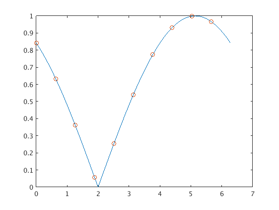
We want to evaluate the interpolating function on a finer mesh with mp points. We extend the a and b vectors with zeros for higher frequencies.
These padded coefficient vectors ap and bp still represent the same interpolating function, but now the inverse transform yields values on a finer mesh.
K = (mp-m)/2;
ap = [a;zeros(K,1)];       % extend a and b vector with K zeros
bp = [b;zeros(K,1)];

Up = inv_cossin_transform(ap,bp);  % this gives now function values on fine grid with 1000 points tp

plot(tp,Up); hold off; axis tight
legend('u(t)', 'interpolation points', 'p(t)','Location','best')
hold off