Example for Principal Component Analysis: Protein Consumption in Europe
Contents
Read Data Set
This data set shows nutrition data for different types of protein in European countries around 1970.
We want to understand in which way nutrition is different in different countries
Each of the 25 countries has 9 protein values, so we have 25 data points in R^9. Since we cannot make a plot in R^9 we want to find the 2-dimensional subspace which is closest to the data points. We can then plot the orthogonal projection of the data points onto this 2-dimensional subspace.
T = readtable('proteindata.txt','Delimiter','\t','HeaderLines',6,'ReadRowNames',true) % 'Table' data type in Matlab
data = table2array(T);                       % numbers as Matlab array
countrynames = T.Properties.RowNames;        % cell arrays of country names and protein names
proteinnames = T.Properties.VariableNames;
T =
                 RedMeat    WhiteMeat    Eggs    Milk    Fish    Cereals    Starch    Nuts    FruitVeg
                 _______    _________    ____    ____    ____    _______    ______    ____    ________
    Albania      10.1        1.4         0.5      8.9     0.2    42.3       0.6       5.5     1.7
    Austria       8.9         14         4.3     19.9     2.1      28       3.6       1.3     4.3
    Belgium      13.5        9.3         4.1     17.5     4.5    26.6       5.7       2.1       4
    Bulgaria      7.8          6         1.6      8.3     1.2    56.7       1.1       3.7     4.2
    Czechosl.     9.7       11.4         2.8     12.5       2    34.3         5       1.1       4
    Denmark      10.6       10.8         3.7       25     9.9    21.9       4.8       0.7     2.4
    EGermany      8.4       11.6         3.7     11.1     5.4    24.6       6.5       0.8     3.6
    Finland       9.5        4.9         2.7     33.7     5.8    26.3       5.1         1     1.4
    France         18        9.9         3.3     19.5     5.7    28.1       4.8       2.4     6.5
    Greece       10.2          3         2.8     17.6     5.9    41.7       2.2       7.8     6.5
    Hungary       5.3       12.4         2.9      9.7     0.3    40.1         4       5.4     4.2
    Ireland      13.9         10         4.7     25.8     2.2      24       6.2       1.6     2.9
    Italy           9        5.1         2.9     13.7     3.4    36.8       2.1       4.3     6.7
    Netherl.      9.5       13.6         3.6     23.4     2.5    22.4       4.2       1.8     3.7
    Norway        9.4        4.7         2.7     23.3     9.7      23       4.6       1.6     2.7
    Poland        6.9       10.2         2.7     19.3       3    36.1       5.9         2     6.6
    Portugal      6.2        3.7         1.1      4.9    14.2      27       5.9       4.7     7.9
    Romania       6.2        6.3         1.5     11.1       1    49.6       3.1       5.3     2.8
    Spain         7.1        3.4         3.1      8.6       7    29.2       5.7       5.9     7.2
    Sweden        9.9        7.8         3.5     24.7     7.5    19.5       3.7       1.4       2
    Switzerl.    13.1       10.1         3.1     23.8     2.3    25.6       2.8       2.4     4.9
    UK           17.4        5.7         4.7     20.6     4.3    24.3       4.7       3.4     3.3
    USSR          9.3        4.6         2.1     16.6       3    43.6       6.4       3.4     2.9
    WGermany     11.4       12.5         4.1     18.8     3.4    18.6       5.2       1.5     3.8
    Yugosl.       4.4          5         1.2      9.5     0.6    55.9         3       5.7     3.2
Perform Principal Component Analysis
We see that
- the first principal component captures 71% of the variance
- the first 2 principal components capture 85% of the variance
- the first 3 principal components capture 92% of the variance
Z = data';                        % use transpose matrix: columns of Z are protein values for each country
                                  % We obtain 25 data points in R^9
X = Z - mean(Z,2)*ones(1,25);     % subtract the row mean from each row
Variance = norm(X,'fro')^2        % Variance is 25 times the variance of the data
[U,S,V] = svd(X);
s = diag(S)                       % singular values
Variance2 = sum(s.^2)             % same as Variance
cumsum(s.^2)/sum(s.^2)            % amount of variance which is captured by 1,2,3,... principal components
Variance =
   5.2434e+03
s =
   61.0378
   27.1435
   19.3764
   14.1282
    9.3337
    7.6349
    6.1125
    4.1419
    2.4599
Variance2 =
   5.2434e+03
ans =
    0.7105
    0.8510
    0.9226
    0.9607
    0.9773
    0.9884
    0.9956
    0.9988
    1.0000
First two principal components
We choose the columns of U as the new basis of our 9-dimensional data space. This is an orthonormal change of basis: c = U'*x.
For our data points we obtain C = U'*X = S*V.
We then plot the projection of the data points onto the span of the first two columns u1,u2.
Each of the data points is approximated by c1*u1 + c2*u2, and we plot the points (c1,c2).
The horizontal green line corresponds to the best 1-dimensional subspace approximating the data.
The original unit vectors in the 9-dimensional data space (for 'RedMeat','WhiteMeat',etc.) become after the projection the columns of U(:,1:2)', i.e., the first two rows of U. We plot these vectors in red (with a scaling factor so that we can see them).
C = S(1:2,1:2)*V(:,1:2)';         % (c1,c2) coordinates of data points, same as U(:,1:2)'*X
W = 20*U(:,1:2);                  % projected unit vectors, scaled with factor 20

plot(C(1,:),C(2,:),'o'); hold on  % plot (c1,c2)
text(C(1,:),C(2,:),countrynames,'FontSize',7,'VerticalAlignment','bottom');  % label with country name
z = zeros(1,9);

plot([z;W(:,1)'],[z;W(:,2)'],'r');  % plot projected unit vectors for proteins, label with protein names
text(W(:,1),W(:,2),proteinnames,'FontSize',7,'VerticalAlignment','bottom','HorizontalAlignment','right','color','red');
grid on; axis equal
ax = axis; plot(ax(1:2),[0 0],'g',[0 0],ax(3:4),'g')   % draw horizontal and vertical axes in green
xlabel('c_1'); ylabel('c_2')
hold off
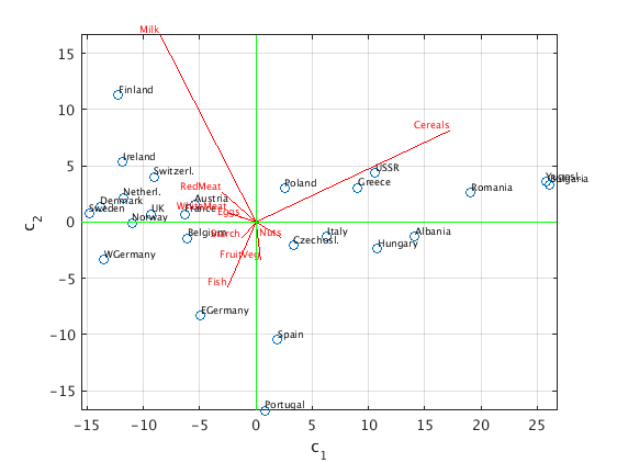
Interpretation of the result
- The first principal component c1 (along horizontal green line) increases with cereal consumption, and decreases with white & red meat consumption. Eastern block countries like Bulgaria, Yugoslavia, Romania are far to the right, whereas wealthy western countries like Sweden, Denmark, WGermany are far to the left.
- The second principal component c2 (along vertical green line) increases with milk consumption, and decreases with fish consumption. Finland is at the top (lots of milk, little fish); countries like Portugal, Spain are at the bottom (lots of fish, little milk).
First three principal components
We now use the first three principal components and plot the points (c1,c2,c3).
We show two "side views" of this 3d picture: c3 vs c1, and c3 vs c2.
C = S(1:3,1:3)*V(:,1:3)';          % (c1,c2,c3) coordinates of data points, same as U(:,1:3)'*X
W = 20*U(:,1:3);                   % projected unit vectors, scaled with factor 20

figure(1)                          % plot (c1,c3)
plot(C(1,:),C(3,:),'o'); hold on
text(C(1,:),C(3,:),countrynames,'FontSize',7,'VerticalAlignment','bottom');
z = zeros(1,9);
plot([z;W(:,1)'],[z;W(:,3)'],'r'); % plot projected unit vectors for proteins
text(W(:,1),W(:,3),proteinnames,'FontSize',7,'VerticalAlignment','bottom','HorizontalAlignment','right','color','red');
grid on; axis equal
ax = axis; plot(ax(1:2),[0 0],'g',[0 0],ax(3:4),'g') % draw horizontal and vertical axes in green
xlabel('c_1'); ylabel('c_3')
hold off

figure(2)                           % plot(c2,c3)
plot(C(2,:),C(3,:),'o'); hold on
text(C(2,:),C(3,:),countrynames,'FontSize',7,'VerticalAlignment','bottom');
z = zeros(1,9);
plot([z;W(:,2)'],[z;W(:,3)'],'r');  % plot projected unit vectors for proteins
text(W(:,2),W(:,3),proteinnames,'FontSize',7,'VerticalAlignment','bottom','HorizontalAlignment','right','color','red');
grid on; axis equal
ax = axis; plot(ax(1:2),[0 0],'g',[0 0],ax(3:4),'g') % draw horizontal and vertical axes in green
xlabel('c_2'); ylabel('c_3')
hold off
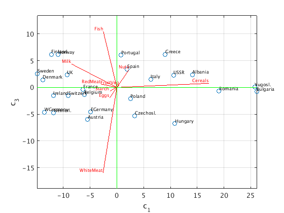
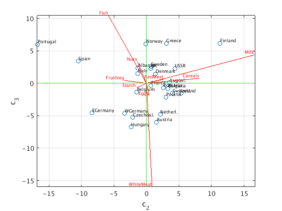
Interpretation of the result
We see that the third principal component c3 increases with fish, and decreases with white meat. Portugal, Norway, Greece, Finland are at the top (lots of fish, little white meat); Hungary and Austria are at the bottom (lots of white meat, little fish).