Example for Principal Component Analysis (PCA): Iris data
Contents
The Iris data set
Download the file irisdata.txt.
We have 150 iris flowers. For each flower we have 4 measurements
- sepal length, sepal width, petal length, petal width
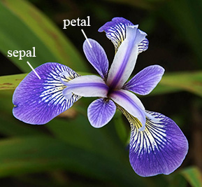
giving 150 points 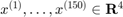 .
.
The flowers belong to three different species (array spec) (shown as blue, green, yellow dots in the graphs below):
- 0: setosa (blue dots), 1: versicolor (green dots), 2: virginica (yellow dots)
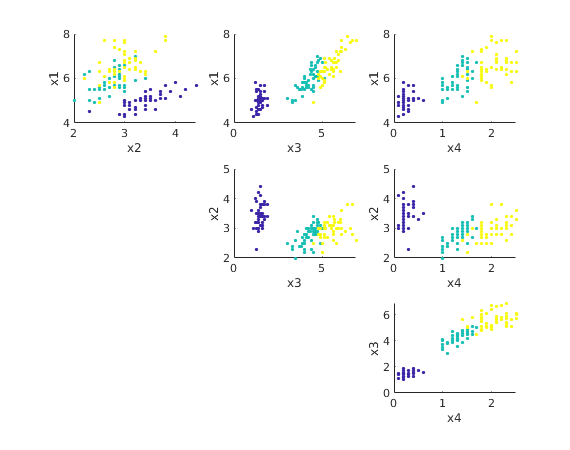
The data points are in 4 dimensions. We can get an idea of the data by plotting  vs
vs  for all 6 combinations of j,k.
Note that species 0 (blue dots) is clearly separated in all these plots, but species 1 (green dots) and species 2 (yellow dots) are harder to separate.
For future measurements of flowers we want to find a way to determine the species from the measurements.
Obviously each of these six 2D plots shows only a small part of the information. Can we make a 2D plot which captures most of the information?
load irisdata.txt           % array of size 150 x 5

X = irisdata(:,1:4)';       % 150 columns of length 4
spec = irisdata(:,5)';      % vector of length 150 with species (0,1,or 2)
n = size(X,2);

figure(1)                   % plot x_i vs x_j for all combinations of i,j
for i=1:4
  for j=1:i-1
     subplot(3,3,(i-1)+3*(j-1))
     scatter(X(i,:),X(j,:),7,spec,'filled')
     xlabel(sprintf('x%g',i)); ylabel(sprintf('x%g',j))
  end
end
Performing Principal Component Analysis (PCA)
We first find the mean vector Xm and the "variation of the data" (corresponds to the variance) We subtract the mean from the data values.
We then apply the SVD. The singular values  are 25, 6.0, 3.4, 1.9. The total variation is
  .
.
Xmean = mean(X,2)           % find mean
A = X - Xmean*ones(1,n);    % subtract mean from each point
rho = norm(A,'fro')^2       % total variation of data

[U,S,V] = svd(A,'econ');    % find singular value decomposition
sigma = diag(S)             % singular values

rho = norm(sigma)^2         % gives same variation as above
Xmean =
       5.8433
        3.054
       3.7587
       1.1987
rho =
       680.82
sigma =
        25.09
       6.0079
       3.4205
       1.8785
rho =
       680.82
Plotting the first two components
We find the coefficients of the data vectors with respect to the singular vectors  .
.
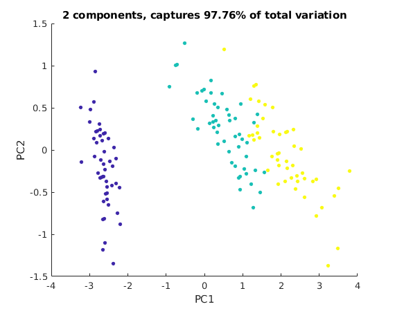
We then plot the first 2 coefficients of each data point.
This 2D view captures almost 98% of the variation of the original data points.
We can now better see how to separate species 1 (green dots) from species 2 (yellow dots).
We can now try to draw some boundaries between the yellow, green, and blue regions. This allows us to classify flowers from measurements.
C = S(1:3,1:3)*V(:,1:3)';   % first 3 coefficients for each point, same as U(:,1:3)'*A;

q2 = norm(sigma(1:2))^2/rho % part of variation captured by first 2 components
figure(2);
scatter(C(1,:),C(2,:),17,spec,'filled')
xlabel('PC1'); ylabel('PC2')
title(sprintf('2 components, captures %.4g%% of total variation',100*q2))
q2 =
      0.97763
Plotting the first three components
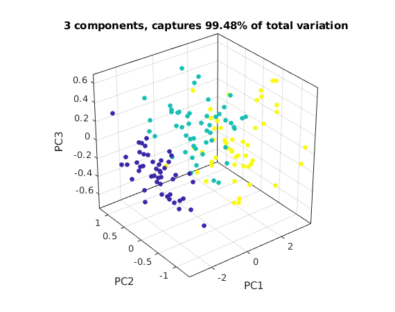
We now plot the first three coefficients of each data point in 3D.
The image below only shows one view. Run this m-file in Matlab, then you can spin the graph around with the mouse to see the points in 3D.
q3 = norm(sigma(1:3))^2/rho   % part of variation captured by first 3 components
figure(3);
scatter3(C(1,:),C(2,:),C(3,:),27,spec,'filled')
nice3dn
xlabel('PC1'); ylabel('PC2'); zlabel('PC3')
title(sprintf('3 components, captures %.4g%% of total variation',100*q3))
% you can rotate and spin this graph with the mouse
q3 =
      0.99482