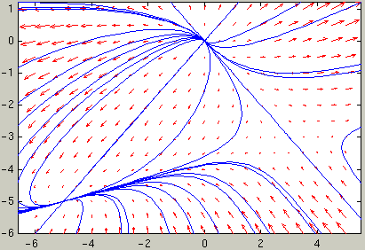
vectfield(g,-6:.5:5,-6:.5:1)
hold on
for a1=-7:2:5
for a2=-7:2:1
[ts,ys] = ode45(g,[0,4],[a1;a2]);
plot(ys(:,1),ys(:,2))
[ts,ys] = ode45(g,[0,-4],[a1;a2]);
plot(ys(:,1),ys(:,2))
end
end

Here we consider the following example of an autonomous system:
y1' = 4y1 + y2 + y1 y2
y2' = y1 + 4 y2 + y22
First define the right hand side function
g of the differential equation as
g = inline('[4*y(1)+y(2)+y(1)*y(2) ;
y(1)+4*y(2)+y(2)^2]','t','y')
To plot the vector field for y1 between -6 and 5 and y2 between -6 and 1 type
vectfield(g,-6:.5:5,-6:.5:1)
To plot a trajectory in the phase plane starting at a point
(a1, a2) at time t=0 for
increasing values of t going from 0 to 4 type
[ts,ys] = ode45(g,[0,4],[a1;a2]);
plot(ys(:,1),ys(:,2))
To plot the trajectory in the phase plane starting at the point
(a1, a2) at time t=0 for
decreasing values of t going from 0 to -4 type
[ts,ys] = ode45(g,[0,-4],[a1;a2]);
plot(ys(:,1),ys(:,2))
To get an idea of the behavior of the ODE, we plot the direction field
and several trajectories together: We can choose e.g. the 35
starting points (a1, a2) with
a1=-7,-5,-3,-1,1,3,5 and a2=-7,-5,-3,-1,1. From each
of those points we plot the trajectory for t going from 0 to 4 and
for t going from 0 to -4:
vectfield(g,-6:.5:5,-6:.5:1)
hold on
for a1=-7:2:5
  for a2=-7:2:1
    [ts,ys] = ode45(g,[0,4],[a1;a2]);
    plot(ys(:,1),ys(:,2))
    [ts,ys] = ode45(g,[0,-4],[a1;a2]);
    plot(ys(:,1),ys(:,2))
  end
end
These commands will generate a number of warning messages (since some solutions don't exist for t in the whole interval [-4,4]) which you can ignore.
From the picture it appears that there are three critical points: A stable node, an unstable node, and a saddle point.
It is convenient to define two functions g1(y1,y1),
g2(y1,y2) containing the right-hand side functions as
follows:
g1 = inline('4*y1+y2+y1*y2','y1','y2')
g2 = inline('y1+4*y2+y2^2','y1','y2')
To find critical points where both g1 and
g2 are zero we use solve:
syms y1 y2
[y1s,y2s] = solve(g1(y1,y2),g2(y1,y2),y1,y2)
This returns
y1s =   [  0]
        [ -5]
        [  3]

y2s =   [  0]
        [ -5]
        [ -3]
Therefore we have found three critical points: (0,0), (-5,-5) and (3,-3).
To find the Jacobian matrix we type
jac = jacobian([g1(y1,y2);g2(y1,y2)],[y1,y2])
This returns the matrix
[   4+y2,   1+y1]
[      1, 4+2*y2]
As an example we will study the second critical point with coordinates
y1s(2)=-5, y2s(2)=-5.
To evaluate the Jacobian at the critical point we substitute
y1s(2) and y2s(2) for y1 and
y2:
jac2 = subs(jac,{y1,y2},{y1s(2),y2s(2)})
which gives the matrix
[ -1, -4]
[  1, -6]
To find the eigenvectors and eigenvalues of this matrix type
[eigvect,eigval] = eig(jac2)
which gives
eigvect =  [ 1, 4]
           [ 1, 1]

eigval =   [ -5,  0]
           [  0, -2]
This means that the eigenvalues are -5 and -2. Hence this critical point is a
stable node. The eigenvector for the first eigenvalue -5 is given by
the first column of the matrix eigvect, it has components 1, 1.
The eigenvector for the second eigenvalue -5 is given by the second column of
the matrix eigvect, it has components 4, 1. Using the
eigenvectors we can sketch by hand the behavior of the trajectories close to
the critical point:
Compare this picture with the trajectories near (-5,-5) in the picture above.
You should try to analyze the other two critical two points by yourself in the same way.