Assignment 2, problem 2

Contents

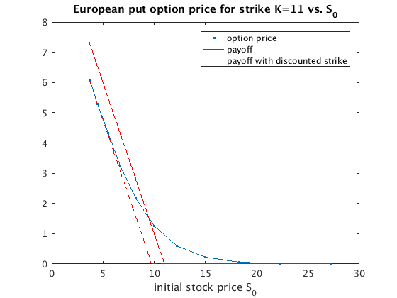
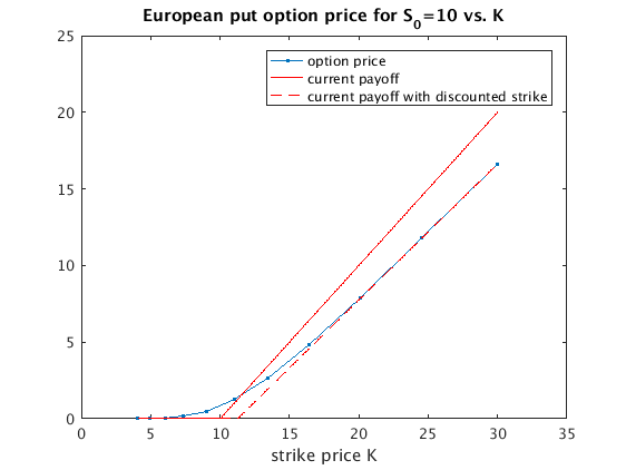
Problem 2(a): European Put Option

S0 = 10; u = 1.1; d = 0.9;  % binomial stock price model
rho = .01;                  % interest rate per period
N = 12;                     % maturity
K = 11;                     % strike

[V0_EP,av] = xbinom_eu_put(rho,S0,u,d,N,K,5);
disp('    S0        V0_EP')
disp([S0*av',V0_EP'])     % table: initial stock price, option price

    S0        V0_EP
    3.6665    6.0958
    4.4813    5.2862
    5.4771    4.3248
    6.6942    3.2494
    8.1818    2.1704
   10.0000    1.2439
   12.2222    0.5896
   14.9383    0.2222
   18.2579    0.0634
   22.3152    0.0128
   27.2741    0.0016

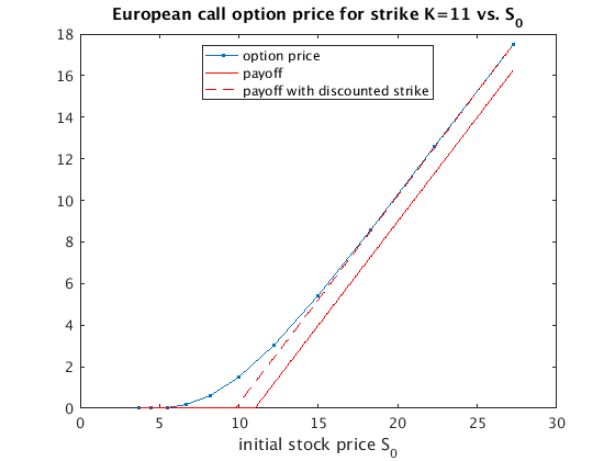
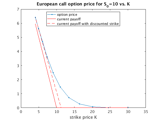
Problem 2(b): European Call Option

[V0_EC,av] = xbinom_eu_call(rho,S0,u,d,N,K,5);
disp('    S0        V0_EC')
disp([S0*av',V0_EC'])     % table: initial stock price, option price

    S0        V0_EC
    3.6665    0.0003
    4.4813    0.0055
    5.4771    0.0399
    6.6942    0.1817
    8.1818    0.5903
   10.0000    1.4820
   12.2222    3.0499
   14.9383    5.3985
   18.2579    8.5594
   22.3152   12.5661
   27.2741   17.5138

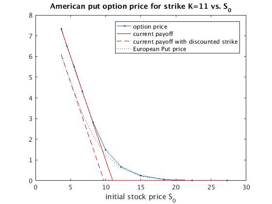
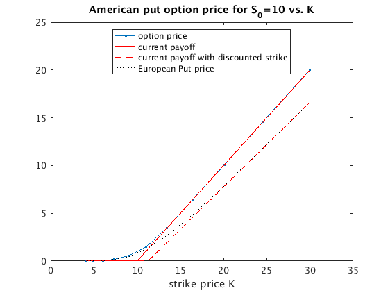
Problem 2(c): American Put Option

We see that the American Put option price is larger than the European Put option price. In the graphs the black dotted curve is the European Put price.

[V0_AP,av] = xbinom_am_put(rho,S0,u,d,N,K,5);
disp('    S0        V0_AP     V0_EP')
disp([S0*av',V0_AP',V0_EP'])     % table: initial stock price, option price
figure(1); hold on
plot(S0*av,V0_EP,'k:'); hold off;
legend('option price','current payoff','current payoff with discounted strike','European Put price')

figure(2); hold on
plot(K./av,V0_EP./av,'k:'); hold off;
legend('option price','current payoff','current payoff with discounted strike','European Put price','Location','best')

    S0        V0_AP     V0_EP
    3.6665    7.3335    6.0958
    4.4813    6.5187    5.2862
    5.4771    5.5229    4.3248
    6.6942    4.3058    3.2494
    8.1818    2.8182    2.1704
   10.0000    1.4895    1.2439
   12.2222    0.6668    0.5896
   14.9383    0.2415    0.2222
   18.2579    0.0669    0.0634
   22.3152    0.0132    0.0128
   27.2741    0.0016    0.0016

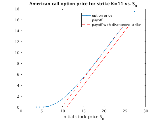
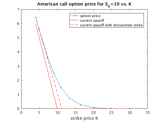
Problem 2(d): American Call Option

We see that the American Call option price is the same as the European Call option price.

[V0_AC,av] = xbinom_am_call(rho,S0,u,d,N,K,5);
disp('    S0        V0_AC     V0_EC')
disp([S0*av',V0_AC',V0_EC'])     % table: initial stock price, option price

    S0        V0_AC     V0_EC
    3.6665    0.0003    0.0003
    4.4813    0.0055    0.0055
    5.4771    0.0399    0.0399
    6.6942    0.1817    0.1817
    8.1818    0.5903    0.5903
   10.0000    1.4820    1.4820
   12.2222    3.0499    3.0499
   14.9383    5.3985    5.3985
   18.2579    8.5594    8.5594
   22.3152   12.5661   12.5661
   27.2741   17.5138   17.5138

Published with MATLAB® R2016a