Example for Stock and Option Prices

Contents

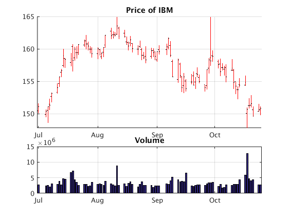
Stock prices

We look at IBM stock prices for July to October 2016.

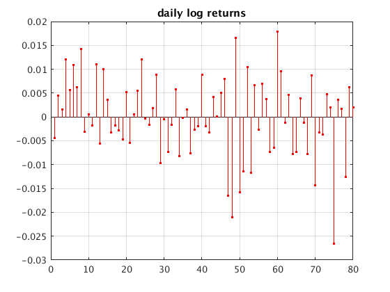
Compute the log returns from the daily closing prices.

[so,sc] = get_stock_plot('IBM',[2016 7],[]); % from July 1 2016 to now
                                            % sc are closing prices

r = log(sc(2:end)./sc(1:end-1));            % daily log returns
figure(2); stem(r,'r.'); grid on
title('daily log returns')

Option prices

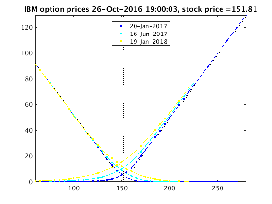
Get the current IBM option prices and plot them:

data = getOptionPrices('IBM')
option_plot(data)

data = 
           sym: 'IBM'
          time: 26-Oct-2016 19:00:03
    stockprice: 151.81
           opt: [1x3 struct]

Call option prices with maturity June 2017

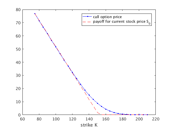
We get option data with 3 expiration dates. For the 2nd expiration date: make a table and a plot of call option price vs. strike

S0 = data.stockprice   % current stockprice
option = data.opt(2);  % option prices for 2nd expiration date
option.expir           % expiration date
K = option.cstrike;    % vector of strike values for call option
V = option.cprice;     % vector of call option prices
[K',V']                % table of call option prices
plot(K,V,'.-',K,max(S0-K,0),'r--')
xlabel('strike K')
legend('call option price','payoff for current stock price S_0')

S0 =
       151.81
ans = 
   16-Jun-2017
ans =
           75         76.8
           80       71.575
           85       66.675
           90       61.625
           95        56.65
          100        51.75
          105       46.625
          110        41.55
          115       36.975
          120         32.4
          125       27.725
          130       23.225
          135       18.875
          140       15.075
          145       11.825
          150        8.825
          155        6.375
          160        4.425
          165         2.87
          170         1.78
          175         1.08
          180         0.63
          185        0.355
          190         0.19
          195        0.115
          200         0.07
          205         0.05
          210         0.04

Find implied volatility

For the strike K0=150 use the call option price to find the implied volatility sigma.

We obtain an implied volatility sigma=16.4%.

T = years(option.expir-data.time) % time between expir. of option and time of data in years
K0 = 150;
i = find(K==K0)         % find i with K(i)=150
V0 = V(i)               % corresponding option price
rc = 0;                 % use interest rate rc=0
f = @(sigma) BlackScholes(S0,K0,rc,sigma,T)-V0;
sigma = fzero(f,0.3)    % find implied volatility sigma

T =
      0.63576
i =
    16
V0 =
        8.825
sigma =
      0.16442

Published with MATLAB® R2016a