Curve fitting example 1
Contents
find speed: fit data with linear function y = c1*1 + c2*t
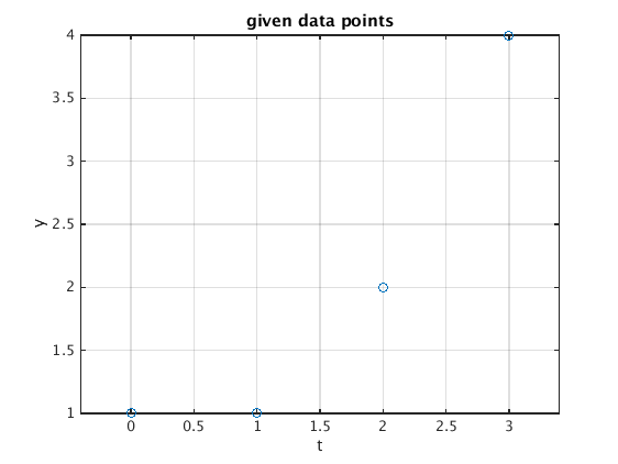
We assume a car is driving with constant speed. In order to find the speed we measure the position y at four t-values.
                         % given data:
t = [0;1;2;3];           %   t-values
y = [1;1;2;4];           %   y-values

data = [t,y]             % table of given t and y values
plot(t,y,'o')            % plot given data points
xlabel('t');ylabel('y')
grid on; axis equal; title('given data points')

A = [t.^0,t]             % matrix A
data =
     0     1
     1     1
     2     2
     3     4
A =
     1     0
     1     1
     1     2
     1     3
Solve normal equations
The normal equations are a 2 by 2 linear system.
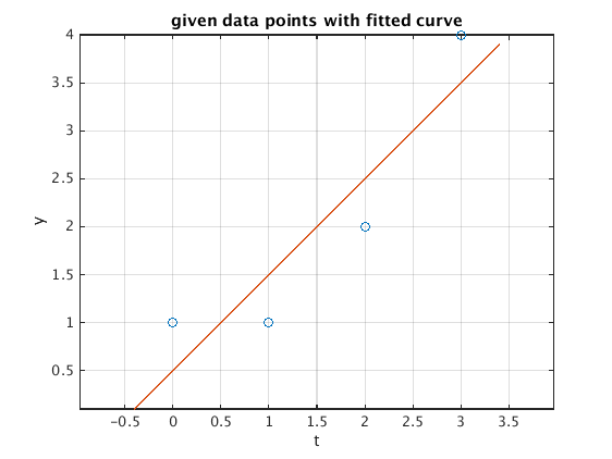
Result: The best least squares fit is y = 0.5 + 1*t, so the estimated speed is 1.
M = A'*A
g = A'*y
c = M\g

tp = (-0.4:.1:3.4)';     % t-values for plotting curve
yp = [tp.^0,tp]*c;       % y-values for fitted curve

plot(t,y,'o',tp,yp)      % plot data points together with fitted curve
xlabel('t');ylabel('y')
grid on; axis equal; title('given data points with fitted curve')
M =
     4     6
     6    14
g =
     8
    17
c =
    0.5000
    1.0000
Check residual vector
Find the norm of the residual vector r. Check that r is really orthogonal on the columns of the matrix A.
r = A*c - y              % residual vector
norm_r = norm(r)         % norm
A'*r                     % dot product of columns of A with r
r =
   -0.5000
    0.5000
    0.5000
   -0.5000
norm_r =
     1
ans =
     0
     0