Solving a nonlinear system with the Newton method and fsolve

Contents

You need to download an m-file

Download the following m-file and put it in the same directory with your other m-files:

Define function f(x) and Jacobian f'(x)

Here we use @-functions in Matlab. For more complicated functions one can define the functions in separate m-files f.m and fp.m .

f = @(x) [ 2*x(1)+x(1)*x(2)-2 ; ...
           2*x(2)-x(1)*x(2)^2-2 ];
fp = @(x) [ 2+x(2) , x(1) ; ...
           -x(2)^2 , 2-2*x(1)*x(2) ];

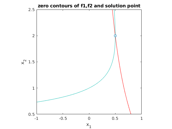
Plot zero contours of the functions f1, f2

The points where f1(x)=0 are shown in green, the points where f2(x)=0 are shown in red. We want to find the solution x at the intersection of the green and red curve.

zerocont2(f,[-1 1 .5 2.5]); hold on
title('zero contours of f1 (red) and f2 (green)')

Perform Newton iteration starting with [0;0]

format long g        % show all digits
x = [0;0];           % initial guess
while 1
  b = f(x);          % evaluate f
  A = fp(x);         % evaluate Jacobian
  d = -A\b;          % solve A*d = -b
  x = x + d
  if norm(d)<=1e-13  % stop iteration if norm(d)<=StepTolerance
    break
  end
end

plot(x(1),x(2),'o'); hold off %    mark solution point with 'o'
title('zero contours of f1,f2 and solution point')

x =
     1
     1
x =
     0
     3
x =
                       0.4
                       2.8
x =
         0.483870967741935
          1.99354838709677
x =
          0.50009892401114
          1.99939860092483
x =
         0.499999985726356
          1.99999999518732
x =
                       0.5
                         2
x =
                       0.5
                         2

Find errors

We see that we have convergence of order 2: the number of correct digits doubles with each iteration.

format short e
xs = x;              % xs is exact solution which we just found
x = [0;0];           % initial guess
for i=1:10
  b = f(x);          % evaluate f
  A = fp(x);         % evaluate Jacobian
  d = -A\b;          % solve A*d = -b
  x = x + d;
  disp(norm(x-xs,Inf))    % print infinity-norm of error
end

     1
     1
   8.0000e-01
   1.6129e-02
   6.0140e-04
   1.4274e-08
     0
     0
     0
     0

Solving the nonlinear system with fsolve

You can solve a nonlinear system f(x)=0 using fsolve. This has the following advantages:

format long g

f = @(x) [ 2*x(1)+x(1)*x(2)-2 ; 2*x(2)-x(1)*x(2)^2-2 ];  % define f
x0 = [0;0];                                              % initial guess
xs = fsolve(f,x0)                                        % find solution xs

Equation solved.

fsolve completed because the vector of function values is near zero
as measured by the default value of the function tolerance, and
the problem appears regular as measured by the gradient.



xs =
         0.500000000000263
          1.99999999997706

Using optimset to get a more accurate solution

We check the computed solution xs and find norm(f(xs))=1e-11.

By default fsolve uses TolX=1e-6 and TolFun=1e-6.

We can obtain a more accurate result xnew by specifying lower values for TolX, TolFun.

fsolve iterates until the last step is less than TolX, or norm(f(xs)) is less than TolFun

norm_fxs = norm(f(xs))

opt = optimset('TolFun',1e-14,'TolX',1e-14);  % you need to use optimset to specify options
xnew = fsolve(f,x0,opt)
norm_fxnew = norm(f(xnew))

norm_fxs =
      1.04713608404361e-11

Equation solved.

fsolve completed because the vector of function values is near zero
as measured by the selected value of the function tolerance, and
the problem appears regular as measured by the gradient.



xnew =
                       0.5
                         2
norm_fxnew =
     0

Published with MATLAB® R2018a