Euler Method for unstable and stable ODEs
Contents
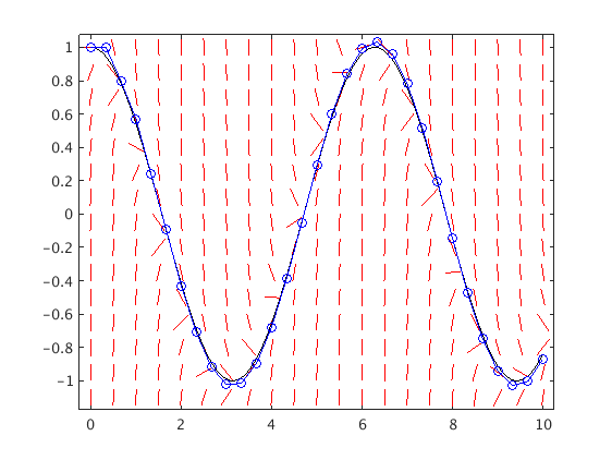
Unstable ODE
Consider the IVP
- y' = y - sin(t) - cos(t)
- y(0) = 1
which has the exact solution y(t)=cos(t). Since f_y=1>0 this is an unstable ODE.
We see that the error grows exponentially with t.
T = 5;
f = @(t,y) y-sin(t)-cos(t);
[ts,ys] = Euler(f,[0,T],1,20);    % use N=20 steps

dirfield(f,0:.2:T,-1.1:.25:6); hold on
tv = linspace(0,T,500);
plot(tv,cos(tv),'k',ts,ys,'bo-'); hold off
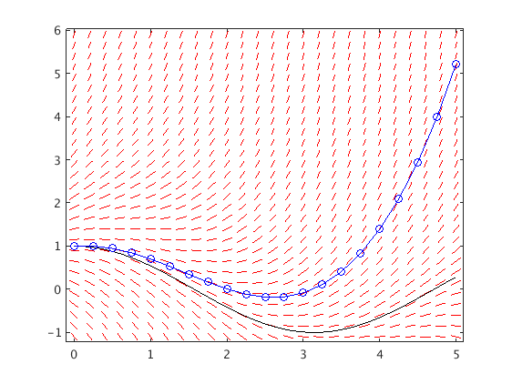
Stable ODE
Consider the IVP
- y' = -y - sin(t) + cos(t)
- y(0) = 1
which has the exact solution y(t)=cos(t). Since f_y=-1<0 this is a stable ODE.
We see that the error stays bounded as t increases.
Here h = 10/20 = 1/2, and f_y=-1, hence the amplification factor has an absolute value < 1:
a = 1 + h*f_y = 1 + 1/2*(-1) = 1/2
T = 10;
f = @(t,y) -y-sin(t)+cos(t);
[ts,ys] = Euler(f,[0,T],1,20);    % use N=20 steps

dirfield(f,0:.4:T,-1.2:.15:1.2); hold on
tv = linspace(0,T,500);
plot(tv,cos(tv),'k',ts,ys,'bo-'); hold off
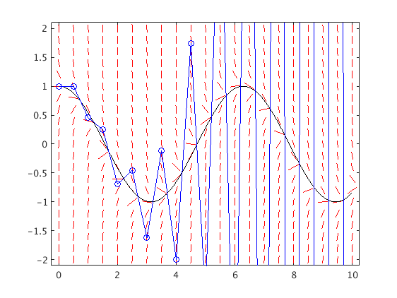
Very stable ODE, large step size
Consider the IVP
- y' = -5*y - sin(t) + 5*cos(t)
- y(0) = 1
which has the exact solution y(t)=cos(t). Since f_y=-5<0 this is a stable ODE.
We see that the error has oscillations which are exponentially growing.
Here h = 10/20 = 1/2, and f_y=-5, hence the amplification factor has an absolute value > 1:
a = 1 + h*f_y = 1 + 1/2*(-5) = -1.5
T = 10;
f = @(t,y) -5*y-sin(t)+5*cos(t);
[ts,ys] = Euler(f,[0,T],1,20);    % use N=20 steps

dirfield(f,0:.5:T,-2:.2:2); hold on
tv = linspace(0,T,500);
plot(tv,cos(tv),'k',ts,ys,'bo-'); hold off
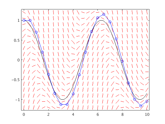
Very stable ODE, small step size
We use 30 instead of 20 time steps. Now the errors are now bounded as t increases.
Here h = 10/30 = 1/3, and f_y=-5, hence the amplification factor has an absolute value < 1:
a = 1 + h*f_y = 1 + 1/3*(-5) = -2/3
T = 10;
f = @(t,y) -5*y-sin(t)+5*cos(t);
[ts,ys] = Euler(f,[0,T],1,30);    % use N=30 steps

dirfield(f,0:.5:T,-1.1:.15:1.1); hold on
tv = linspace(0,T,500);
plot(tv,cos(tv),'k',ts,ys,'bo-'); hold off