Interpolation: Find good approximation from given samples
Contents
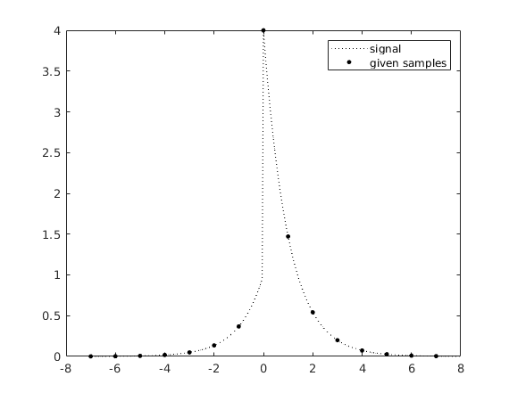
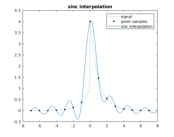
Example: signal with discontinuity, exponential decay
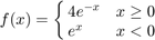
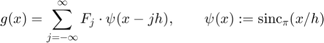
As an example we use the function
Here we use 15 points with a spacing of h=1.
fct = @(x) 4*exp(-x).*(x>=0) + exp(x).*(x<0);

a = -7;
b = 7;
N = 15;                 % number of given points
h = (b-a)/(N-1)         % spacing
x = a + (0:N-1)*h;      % N equidistant nodes where values are given
                        % same as linspace(a,b,N)
F = fct(x);             % discrete signal

m = 20;                 % "upsampling factor": we want to approximate
                        % function at points with spacing h/m
xf = a + (0:m*N-1)*h/m; % points with spacing h/m

plot(xf,fct(xf),'k:',x,F,'k.','MarkerSize',11); hold on
legend('signal','given samples')
h =
     1
Sinc interpolation
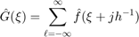
The discrete values  correspond to a linear combination of Dirac deltas
The Fourier transform is the  -periodic function
  , i.e.,
Let  denote the function which is 1 for
  , zero otherwise. We define the interpolating function
  by
by  (low pass filter). Hence the interpolating function is the convolution
  . Since
 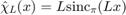 we obtain the "Sinc Interpolation Formula"
Note that  , hence
 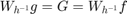 . Therefore sampling
  and at the points
  gives the same values. This corresponds to the fact that
  and
and  for nonzero integers
  .
.
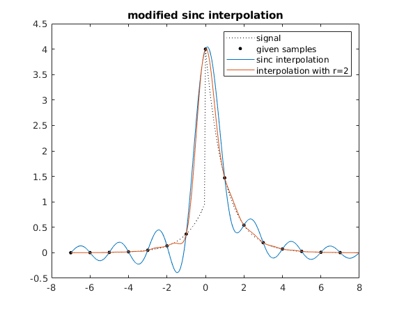
Note that the discontinuity of the signal causes large oscillations in the interpolating function (Gibbs phenomenon). This is due to the fact that  is discontinuous, so has jumps, and has slow decay.
t = (-N*m:N*m)/m*h;
psi = sinc(t/h);
Fu = upsample(F,m);     % Fu = [F(1),0,...,0,F(2),0,...,0,...]
                        % put m-1 zeros after every F(j), Fu has length N*m

                        % conv(Fu,s) computes discrete convolution
                        % conv(Fu,s,'same') gives only values where Fu is given
G = conv(Fu,psi,'same'); % G has length N*m (because of 'same')
xf = a + (0:m*N-1)*h/m;
plot(xf,G)
legend('signal','given samples','sinc interpolation')
title('sinc interpolation')
Modified Sinc Interpolation: Use "smoother low pass filter" in frequency domain
Let  denote the function which is
  for
for  , zero otherwise. Note that the convolution
  gives the "moving average"
  .
.
Let  . Then the convolution
  is piecewise linear and continuous (the derivative has jumps). Its Fourier transform is

Let  . Then the convolution
  is piecewise quadratic with a continous derivative (the second derivative has jumps). Its Fourier transform is

We now use instead of  the smoother function
  . This gives the "Modified Sinc Interpolation Formula"
We use the largest value  :
:
r = 2;                  % use r=2 steps of smoothing: low pass filter chi_L*phi_delta*phi_delta
delta = (1/h)/r;        % we need 0 < delta <= (1/h)/r. We choose largest value.

psir = sinc(t/h).*sinc(delta*t).^r;
Gr = conv(Fu,psir,'same');
plot(xf,Gr);

title('modified sinc interpolation')
legend('signal','given samples','sinc interpolation','interpolation with r=2')