Smoothing and Cutoff Functions

You need to download m-files
Why use "smooth cutoff functions"
Smoothing by convolution
Cutoff functions: simplest choice
Cutoff functions: smoothing with $\phi_\delta$
Cutoff functions: smoothing with $\phi_\delta*\phi_\delta$
Cutoff functions: smoothing with $\phi_\delta*\phi_\delta$ , largest choice of $\delta$

You need to download m-files

You need to download the files Phi.m and Chi.m. Put them in the same directory as your other m-files.

Why use "smooth cutoff functions"

If we only want to use values of $F$ for $x\in [-M,M]$ we could use $F(x)$ inside this interval, and zero outside. But this gives a function with jumps, and the Fourier transform has oscillations and slow decay like $1/|\xi|$ (Gibbs phenomenon).

In several applications we can avoid this problem by using smoother cutoff functions.

reconstructing a function from the Fourier transform $\hat f(\xi)$ for $|\xi|\le M$ .
reconstructing a function from samples .
"short time Fourier transform": analyzing the time dependent behavior of frequencies. We multiply the signal with "windowing functions" $\psi(x)$ , $\psi(x-L)$ , $\psi(x-2L)$ , ... and then compute the Fourier transform of each term $f(x)\psi(x-jL)$ . Since the windowing functions $\psi(x)$ , $\psi(x-L)$ , $\psi(x-2L)$ , ... add up to 1 we can reconstruct the original signal from the Fourier transforms of each term.

Smoothing by convolution

The moving average over an interval of length delta corresponds to convolution with $\phi_\delta$ .

Applying this n times corresponds to convolution with the function $\phi_\delta*\cdots*\phi_\delta$ (convolution of n terms $\phi_\delta$ ).

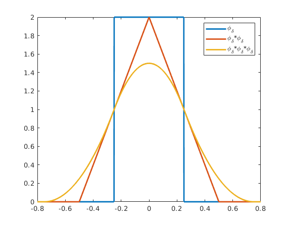
As an example we use delta=.5 and plot the functions $\phi_\delta$ , $\phi_\delta*\phi_\delta$ , $\phi_\delta*\phi_\delta*\phi_\delta$ .

All three functions have integral 1.

In Matlab we use phi(x/delta,n)/delta for $\phi_\delta*\cdots*\phi_\delta$ . The Fourier transform is $\mathrm{sinc}(\pi\delta\xi)^n$ .

d = .5;                  % delta=.5
x = -.8:.001:.8;
plot( x,Phi(x/d)/d, x,Phi(x/d,2)/d, x,Phi(x/d,3)/d ,'LineWidth',2);
legend('\phi_\delta','\phi_\delta*\phi_\delta','\phi_\delta*\phi_\delta*\phi_\delta'); axis tight

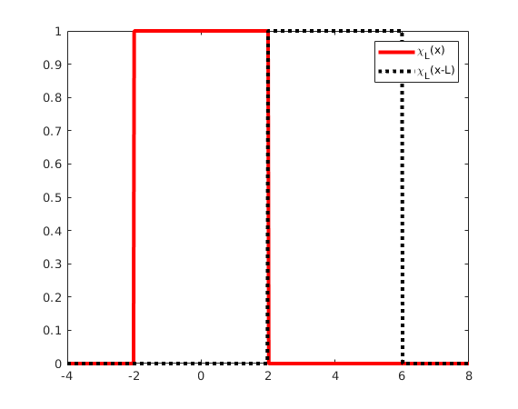
Cutoff functions: simplest choice

The function $\chi_L$ is 1 for $|x|\le L/2$ , zero otherwise.

Here we show for $L=4$ the functions $\chi_L(x)$ , and $\chi_L(x-L)$ . If we add all shifts by integer multiples of $L$ we get the constant function 1.

L = 4;
x = -4:.02:8;
plot( x,Chi(x,L),'r',x,Chi(x-L,L),'k:','LineWidth',3);
legend('\chi_L(x)','\chi_L(x-L)')

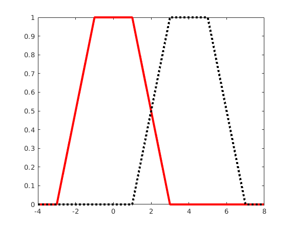
Cutoff functions: smoothing with $\phi_\delta$

Now we use the function $\chi_L*\phi_\delta$ which is piecewise linear and is continuous. This function is zero outside of $[(-L-\delta)/2,(L+\delta)/2]$ . It is one in the interval $[(-L+\delta)/2,(L-\delta)/2]$ .

Here we show for $L=4$ and $\delta=2$ the functions $\chi_L(x)*\phi_\delta$ , and the function shifted by $L$ . If we add all shifts by integer multiples of $L$ we get the constant function 1.

L = 4; d = 2;
x = -4:.02:8;
plot( x,Chi(x,L,d),'r',x,Chi(x-L,L,d),'k:','LineWidth',3);

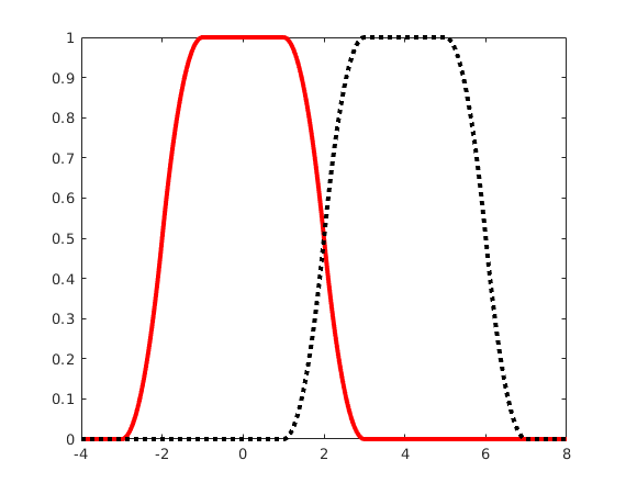
Cutoff functions: smoothing with $\phi_\delta*\phi_\delta$

Now we use the function $\chi_L*\phi_\delta*\phi_\delta$ which is piecewise quadratic, and has a continuous derivative. This function is zero outside of $[-L/2-\delta,L/2+\delta]$ . It is one in the interval $[-L/2+\delta,L/2-\delta]$ .

Here we show for $L=4$ and $\delta=1$ the functions $\chi_L(x)*\phi_\delta$ , and the function shifted by $L$ . If we add all shifts by integer multiples of $L$ we get the constant function 1.

Chi(x,L,delta,n) gives the function $\chi_L*\phi_\delta*\cdots*\phi_\delta$ ( $n$ times $\phi_\delta$ ). Its Fourier transform is $L\mathrm{sinc}(\pi L \xi)\cdot \mathrm{sinc}(\pi\delta\xi)^n$ .

L = 4; d = 1;
x = -4:.02:8;
plot( x,Chi(x,L,d,2),'r',x,Chi(x-L,L,d,2),'k:','LineWidth',3);

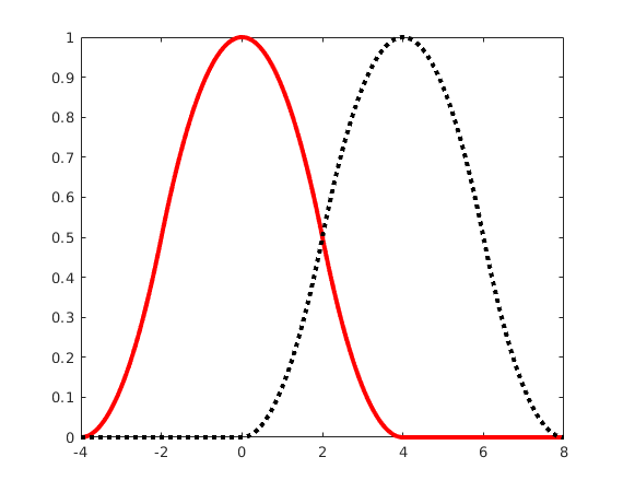
Cutoff functions: smoothing with $\phi_\delta*\phi_\delta$ , largest choice of $\delta$

For Chi(x,L,delta,n) we need $0<\delta\le L/n$ .

We again use $L=4$ and $n=2$ , but now we choose the largest possible value $\delta=L/n=2$ . If we add all shifts by integer multiples of $L$ we get the constant function 1.

L = 4; d = 2;
x = -4:.02:8;
plot( x,Chi(x,L,d,2),'r',x,Chi(x-L,L,d,2),'k:','LineWidth',3);