Example for Principal Component Analysis: Olympic Decathlon 1988
Contents
Read Data Set
This data set contains the results of the 1988 olympic decathlon competition. Each athlete competes in 10 events:
- running: 100m, 110m hurdles, 400m, 1500m
- jumping: long jump, high jump, pole vault
- throwing: javelin, discus, shot put
We want to understand how the athletes differ from each other:
- Are there e.g. athletes which are good at throwing, but bad at jumping (or vice versa)?
- Which events give very similar results (e.g. running 100m and 400m)?
- In which events do the top finishers excel?
We denote the 33 athletes by R1,...,R33 according to their final result (total of the points in 10 events): R1, R2, R3 won gold, silver, bronze.
Each of the 33 athlete was awarded points in 10 events, so we have 33 data points in R^10. Since we cannot make a plot in R^10 we want to find the 2-dimensional subspace which is closest to the data points. We can then plot the orthogonal projection of the data points onto this 2-dimensional subspace.
T = readtable('decathlon1988s.txt','Delimiter','\t','HeaderLines',6,'ReadRowNames',true) % 'Table' data type in Matlab
data = table2array(T);                       % numbers as Matlab array
athletenames = T.Properties.RowNames;        % cell arrays of athlete names and event names
eventnames = T.Properties.VariableNames;
[m,n] = size(data);
T =

  33×10 table

           r100m    longjmp    shotput    highjmp    r400m    r110m    discus    polevlt    javelin    r1500m
           _____    _______    _______    _______    _____    _____    ______    _______    _______    ______

    R1      806       918        819       1061       866      834      855        819        758       752
    R2      890       922        788        776       923      916      754        941        764       725
    R3      821       920        741        776       895      873      739        972        801       790
    R4      947       905        791        831       858      884      763        880        799       648
    R5      899       965        703        915       893      951      727        880        621       718
    R6      856       918        662        776       936      924      689        972        700       835
    R7      821       826        736        859       845      925      699       1132        762       611
    R8      850       802        811        803       899      929      691        849        783       772
    R9      827       842        760        831       854      891      713        880        835       747
    R10     810       881        805        776       880      879      829        972        730       605
    R11     874       950        811        776       817      942      702        849        838       584
    R12     821       896        758        749       860      836      715        819        826       834
    R13     856       883        662        859       898      854      655        910        690       826
    R14     863       903        704        776       917      886      744        702        837       751
    R15     854       922        741        776       869      797      699        819        798       761
    R16     841       833        760        831       820      876      730        880        696       754
    R17     761       755        856        803       757      726      884        849        932       546
    R18     738       814        827        749       822      845      801        880        741       643
    R19     845       823        692        749       911      912      672        849        611       795
    R20     885       830        841        619       829      857      773        880        745       522
    R21     748       900        724        749       815      774      641        790        844       768
    R22     755       818        716        831       787      823      646        819        752       798
    R23     778       833        747        803       804      853      794        731        673       727
    R24     795       807        681        944       816      804      639        790        653       694
    R25     861       869        676        831       827      854      625        760        630       646
    R26     789       774        584        859       891      803      614        790        669       744
    R27     838       809        648        670       879      834      625        819        581       799
    R28     750       816        739        749       762      828      784        790        682       542
    R29     804       790        631        696       898      777      624        731        628       731
    R30     753       835        664        644       849      783      712        760        641       596
    R31     767       635        727        723       758      746      791        790        705       589
    R32     759       682        626        749       801      850      639        617        697       596
    R33     738       859        502        723       782      710      551        645        662       745
Perform Principal Component Analysis
We see that
- the first principal component captures 33.8% of the variance
- the first 2 principal components capture 59.2% of the variance
- the first 3 principal components capture 71.2% of the variance
Z = data';                         % use transpose matrix: columns of Z are event values for each athlete
                                   % We obtain 33 data points in R^10
X = Z - mean(Z,2)*ones(1,m);       % subtract the row mean from each row
Variance = norm(X,'fro')^2         % Variance is 33 times the variance of the data
[U,S,V] = svd(X);
s = diag(S)                        % singular values
Variance2 = sum(s.^2)              % same as Variance
cumsum(s.^2)/sum(s.^2)             % amount of variance which is captured by 1,2,3,... principal components
Variance =

   1.8799e+06


s =

  797.5138
  690.4129
  474.4599
  429.3924
  357.2134
  297.3019
  258.1165
  184.9458
  165.8706
  115.8598


Variance2 =

   1.8799e+06


ans =

    0.3383
    0.5919
    0.7116
    0.8097
    0.8776
    0.9246
    0.9600
    0.9782
    0.9929
    1.0000
First two principal components
We choose the columns of U as the new basis of our 10-dimensional data space. This is an orthonormal change of basis: c = U'*x.
For our data points we obtain C = U'*X = S*V.
We then plot the projection of the data points onto the span of the first two columns u1,u2.
Each of the data points is approximated by c1*u1 + c2*u2, and we plot the points (c1,c2).
The horizontal green line corresponds to the best 1-dimensional subspace approximating the data.
The original unit vectors in the 10-dimensional data space (for events) become after the projection the columns of U(:,1:2)', i.e., the first two rows of U. We plot these vectors in red (with a scaling factor so that we can see them).
C = S(1:2,1:2)*V(:,1:2)';          % (c1,c2) coordinates of data points, same as U(:,1:2)'*X
W = 600*U(:,1:2);                  % projected unit vectors, scaled with factor 600

plot(C(1,:),C(2,:),'o'); hold on   % plot (c1,c2)
text(C(1,:),C(2,:),athletenames,'FontSize',7,'VerticalAlignment','bottom');  % label with athlete name
z = zeros(1,n);

plot([z;W(:,1)'],[z;W(:,2)'],'r'); % plot projected unit vectors for events, label with event names
text(W(:,1),W(:,2),eventnames,'FontSize',7,'VerticalAlignment','bottom','HorizontalAlignment','right','color','red');
grid on; axis equal

xtotvec = ones(n,1)/sqrt(n);       % unit vector for finding sum of points
Wtot = 600*U(:,1:2)'*xtotvec;
% plot([0;Wtot(1)],[0;Wtot(2)],'k:'); % plot vector for "total"

ax = axis; plot(ax(1:2),[0 0],'g',[0 0],ax(3:4),'g')   % draw horizontal and vertical axes in green
xlabel('c_1'); ylabel('c_2')
hold off
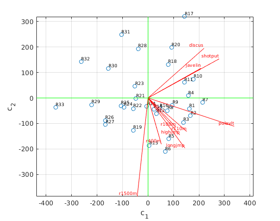
Interpretation of the result
- The first principal component c1 (along horizontal green line) increases most strongly with pole vault, shotput, discus, javelin , and decreases with 1500m. Note that the first principal component is closely related to the total score (the sum of all points, i.e., the inner product of the score vector with the vector (1,...,1)). We see that the top finishers R1, R2, R3, ... are on the right, and the bottom finishers R31, R32, R33 are on the left.
- The second principal component c2 (along vertical green line) increases with the throwing events, and decreases most strongly with 1500m.
First three principal components
We now use the first three principal components and plot the points (c1,c2,c3).
We show two "side views" of this 3d picture: c3 vs c1, and c3 vs c2.
C = S(1:3,1:3)*V(:,1:3)';          % (c1,c2,c3) coordinates of data points, same as U(:,1:3)'*X
W = 600*U(:,1:3);                  % projected unit vectors, scaled with factor 600

figure(1)                          % plot (c1,c3)
plot(C(1,:),C(3,:),'o'); hold on
text(C(1,:),C(3,:),athletenames,'FontSize',7,'VerticalAlignment','bottom');
z = zeros(1,n);
plot([z;W(:,1)'],[z;W(:,3)'],'r'); % plot projected unit vectors for events
text(W(:,1),W(:,3),eventnames,'FontSize',7,'VerticalAlignment','bottom','HorizontalAlignment','right','color','red');
grid on; axis equal
ax = axis; plot(ax(1:2),[0 0],'g',[0 0],ax(3:4),'g') % draw horizontal and vertical axes in green
xlabel('c_1'); ylabel('c_3')
hold off

figure(2)                           % plot(c2,c3)
plot(C(2,:),C(3,:),'o'); hold on
text(C(2,:),C(3,:),athletenames,'FontSize',7,'VerticalAlignment','bottom');
z = zeros(1,n);
plot([z;W(:,2)'],[z;W(:,3)'],'r');  % plot projected unit vectors for events
text(W(:,2),W(:,3),eventnames,'FontSize',7,'VerticalAlignment','bottom','HorizontalAlignment','right','color','red');
grid on; axis equal
ax = axis; plot(ax(1:2),[0 0],'g',[0 0],ax(3:4),'g') % draw horizontal and vertical axes in green
xlabel('c_2'); ylabel('c_3')
hold off
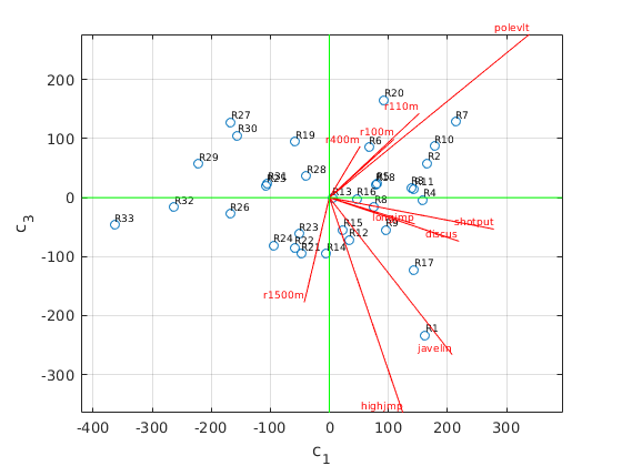
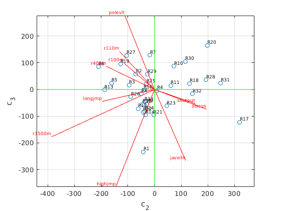
Interpretation of the result
We see that the third principal component c3 increases with running events and pole vault, and decreases most strongly with high jump, javelin, 1500m.