Portugese Hindi
Contents
- What are some challenges in seismic imaging?
- The inverse problem
- Inversion methods
- Examples
- Marmousi example
|
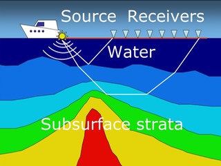
Imagine a boat releasing impulsive sounds waves at equal intervals of time. The pressure waves propagate down to the seabed and then deeper into the earth: they are reflected by both the seabed and from underground layer boundaries. Seismic data are produced by towed receivers which record the amplitudes and times of the reflected signals. Our goal is to build a fast and robust algorithm for finding the sound speeds ("seismic velocities") inside the earth from these data. Careful measurements of the seismic velocity are part of obtaining accurate seismic images showing layers and cracks inside the earth, and are used to determine geologic features, such as the location of oil trapped at the sides of a salt dome, shown here by the red color. |
 |
What are some challenges in seismic imaging?
A location of a point A inside the earth can be described in either of two coordinate systems:
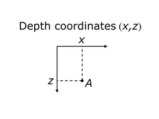
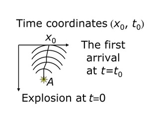
Depth coordinates, on the left above, give a location of a point A inside the earth in terms of its position on the top and depth below. In contrast, time coordinates, shown on the right, think of each point A under the earth's surface as corresponding to a pair (x0, t0): if you imagine a wave starting at point A, x0 is where it first hits the earth's surface, and t0 is the time when it does so. While it may be counterintuitive, seismic data are most naturally first recorded in time coordinates rather than depth coordinates.
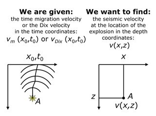
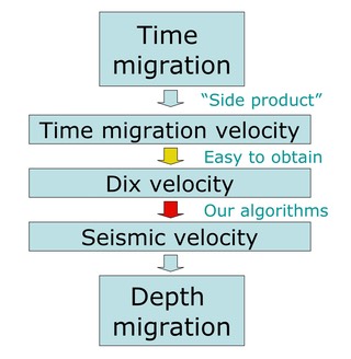
The two main approaches to seismic imaging produce models for the underground velocities: the first is a process called time migration, which takes seismic data in time coordinates, and produces images and time-migration velocities, which are an averaged velocity of a particular type. The second, depth migration, takes seismic data in depth coordinates and produces seismic images in depth coordinates.
|
Time migration
|
Depth migration
|
|
|---|---|---|
|
Adequate for
|
mild lateral velocity
variation |
arbitrary velocity
variation |
|
Implementation
requires |
seismic data
|
seismic data
+ velocity model |
|
Produces images in
|
time coordinates
|
depth coordinates
|
Time migration has the advantage in that it is fast and efficient, however:
- It works best in areas where the seismic velocity depends only on the depth, in other words, the sound speed is constant along horizontal lines. However, most interesting phenomena, including the presence of underground oil, tend to occur in the areas where flat horizontal structures inside the earth are distorted;
- Tranforming these images and information from time coordinates to regular Cartesian (depth) coordinates is subtle and non-obvious in cases where the velocity is not horizontally constant and in fact depends on the lateral coordinates.
- In contrast, depth migration produces images in the regular Cartesian coordinates and can be applied when there is considerable lateral distortion in underground structures. However, one needs to start with seismic velocity in depth coordinates in order to apply depth migration: this seismic velocity is never known, and is typically found by "guessing and trying".
The inverse probelm
For the horizonally constant case the relationship between the seismic velocities and the time migration velocities vm(x, t) was derived by C.H. Dix in 1955:
vDix(x, t) = ( ( t vmig(x, t)2)2 )1/2, where (x, t) are the time coordinates.
In order to use depth migration, we would like to understand how time migration velocities relate to true seismic velocities in the general case of horizontally variable velocity. The Dix velocities vDix(x, t)computed from the time migration velocities vm(x, t) by the formula above serve as a more convenient input. Ultimately, we are faced with an inverse problem:
Inversion methods
We have done the following:
- We have produced a theoretical relation between the time migration velocity and the true seismic velocity in 2D and 3D: we have found that the two are linked through a certain thing called geometrical spreading Q. In 2D this relationship is
- Second, using M. M. Popov's equations for the time evolution of Q and our relationship above, we have derived a nonlinear elliptic PDE for Q in the time coordinates.
- At the earth surface Q = 1 and Qt = 0. Therefore, the physical setting allows us to pose only the Cauchy problem for this PDE which is well-known to be ill-posed. Furthermore, this PDE illuminates the high sensitivity of the problem. The coefficients depend not only of the input (the Dix velocity) but also on its first and second derivatives.
v(x, t) = vDix(x, t)/|Q(x, t)|.
(QtvDix-2Q-2)t = - vDix-1Q-1( (vDixQ)xQ-1)x.
Nonetheless we have attempted a regularized reconstruction for a short enough interval of time. (The seismic data are typically acquired only up to 2 seconds and up to 5 km in depth.) We have found two ways to solve this PDE.
- We develop a finite difference time-marching numerical scheme and compute a solution on the required interval of time. Our numerical scheme is motivated by the Lax-Friedrichs method for hyperbolic conservation laws.
- Second, we adjust a spectral Chebyshev method \cite{boyd} for the problem in-hand. We truncate the Chebyshev series to cut off the growing high harmonics in this case.
We have shown that these schemes work because of the following reasons
- special input,
- special initial data,
- suppression/truncation of the high harmonics,
- solving the problem only on a short interval of time such that the growing low harmonics do not have enough time to develop.
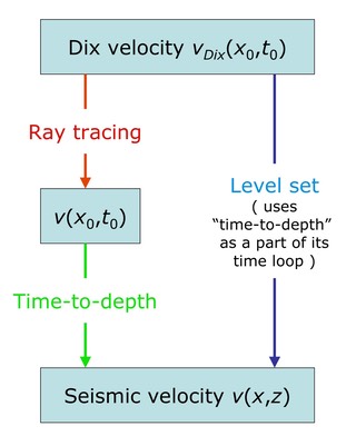
Once we obtain Q we obtain the seismic velocity v in the time coordinates. The next step is to convert the seismic velocity to depth coordinates. To do this we have developed an efficient, Dijkstra-like time-to-depth conversion algorithm. It solves the Eikonal equation with an unknown right-hand side: it does this by systematically building the velocity field by coupling the Eikonal equation with an orthogonality relation. Its motivation and a building block was the fast marching method. This algorithm is considerably faster and more robust than existing techniques. However, because we are required to solve two coupled equations simultaneously in order to build the seismic velocity in depth coordinates, a very subtle issue arises as to whether one can maintain causality in systematically building the solution. After an exhausting six months, the answer turns out to be "yes".
We generalize the PDE and our finite difference numerical scheme to 3D, and test our numerical techniques on a collection of synthetic examples, demonstrating that we are able to restore the seismic velocity quite accurately. Results are compared with the standard Dix estimate, and demonstrate that the Dix estimate might differ qualitatively from the original velocity while our correction gives a significant and qualitative improvement to the Dix estimate. Our test on the smoothed Marmousi data confirms the effectiveness of the proposed approach.
Examples
 |
 |
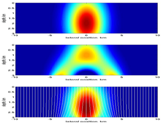
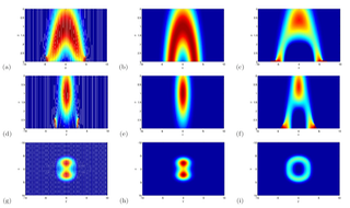
| Symmetric Gaussian anomaly.
Top: the exact velocity. Middle: the input: the Dix Velocity. Bottom: the reconstructed velocity and the rays. |
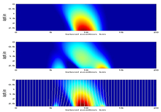
Asymmetric Gaussian anomaly. Top: the exact velocity. Middle: the input: the Dix velocity. Bottom: the reconstructed velocity and the rays. |
 |
 |
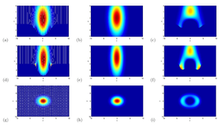
| 3D Gaussian anomaly. Top row: xz-plane; Middle row: yz-plane; Bottom row: xy-plane at 2.55 km in depth. 1st column: the reconstructed velocity; 2nd column: the exact velocity; 3rd column: the Dix velocity. |
3D arch-shaped Gaussian anomaly. Top row: xz-plane; Middle row: yz-plane; Bottom row: xy-plane at 2 km in depth. 1st column: the reconstructed velocity; 2nd column: the exact velocity; 3rd column: the Dix velocity. |
Marmousi example
Slides
References
-
Seismic Velocity Estimation from Time Migration , Cameron, M. K., Fomel, S. B., Sethian, J. A., Inverse Problems, Vol 23, #4, Aug. 2007, p. 1329. -
Seismic velocity estimation and time-to-depth conversion of time- migrated images, Cameron, M.K., Fomel, S., Sethian, J.A., (SVIP 1.7), SEG conference 2006, New Orleans, LA -
Seismic Velocity Estimation from Time Migration, Cameron, M.K., thesis, ProQuest, 2007 -
Time-to-depth conversion and seismic velocity estimation using time-migration velocity, Cameron, M.K., Fomel, S.B., Sethian, J.A., Geophysics, Vol. 73, VE205 (2008) -
Inverse problem in seismic imaging, Maria Cameron, Sergey Fomel, James Sethian, PAMM, Vol. 7, Issue 1, Date: December 2007, Pages: 1024803-1024804 -
Analysis and Algorithms for a Regularized Cauchy Problem arising from a Nonlinear Elliptic PDE for Seismic Velocity Estimation, Cameron, M.K., Fomel, S.B., Sethian, J.A., J. of Comp. Phys., Vol. 228, pp. 7388-7411, 2009 -
Level Set Methods and Fast Marching Methods, James Sethian's web page