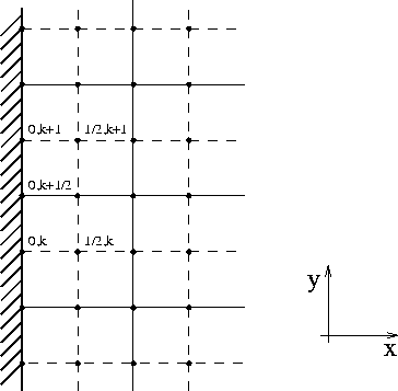
Figure 1.4.10: Two dimensions - left boundary

Figure 1.4.10: Two dimensions - left boundary
We distinguish between inflow (![]() ),
and outflow (
),
and outflow (![]() ), boundary cells.
), boundary cells.
In inflow boundary cells, we reconstruct a constant interpolant
from the
prescribed point-values at these boundaries,
![]()
This reconstruction is then used to build the approximate solution at time ![]() in the interior cells. At the next-time step,
in the interior cells. At the next-time step, ![]() , the
cell-averages at these
boundary cells are defined according to the prescribed point-values as
, the
cell-averages at these
boundary cells are defined according to the prescribed point-values as
![]()
We now turn to the outflow boundary cells.
Here, we extrapolate the data from the interior of the
domain, up to the boundary. First, we determine the discrete slope
in the x-direction,
![]() . This slope is then used to extrapolate the cell-average up
to the boundary,
. This slope is then used to extrapolate the cell-average up
to the boundary,
![]()
which is then used to predict the mid-value,
![]() .
Here
.
Here
![]()
The discrete slope in the y-direction, ![]() , is computed
in that boundary cell
in an analogous way to the interior computation.
In summary, the staggered average at time
, is computed
in that boundary cell
in an analogous way to the interior computation.
In summary, the staggered average at time ![]() is given by
is given by

This concludes the boundary treatment of the left boundary.
Similar expressions hold for the other three boundaries.
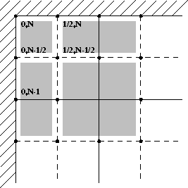
We now turn to the corners and as a prototype, consider the upper-left corner (see Figure 1.4.11). In the corner we repeat the previous boundary treatment with one simple modification. The main difference regarding the boundary scheme in the corner is based on the number of different possible inflow/outflow configurations in that corner.

Figure 1.4.11: Upper-left corner
Computationally, the most complicated case is when the flow
in that upper-left corner is outflow in both directions. In this case,
the staggered average at time ![]() ,
, ![]() ,
is computed according to
,
is computed according to


The cell-average in the north-west edge of Figure 1.4.11
in time ![]() , is given in this outflow-outflow case by
the corrector step
, is given in this outflow-outflow case by
the corrector step

When one of the boundaries is inflow, we have ![]() , and
, and
![]() (- the prescribed
pointvalues at the corner).
(- the prescribed
pointvalues at the corner).
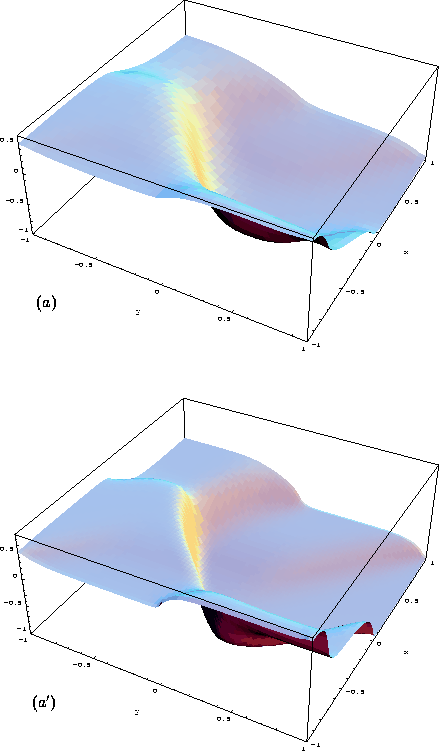
As an example, we we approximate a solution to the
two-dimensional Burgers equation
![]()
subject to the initial conditions,

and augmented with boundary conditions at the inflow boundaries which are equal to the initial values at these same boundaries. Figures 1.4.12 show the evolution of the solution in time for mesh sizes 41*41 and 81*81. Again, we note that there are no spurious oscillations at the boundaries, oscillations that are inherent with a naive treatment of inflow boundaries.

Figure 1.4.12: The 2D IBVP Burgers equation: T=1. (a) N=41, (a') N=81