Central schemes in two space dimensions

Following the one dimensional setup, one can derive a non-oscillatory, two-dimensional central scheme. Here we sketch the construction of the second-order two-dimensional scheme following [16] (see also [2],[1]). For the two-dimensional third-order accurate scheme, we refer to [24].

We consider the two-dimensional hyperbolic system of conservation laws
 
To approximate a solution to (1.4.34), we start with a two-dimensional linear reconstruction

Here, the discrete slopes in the x and in the y direction approximate the corresponding derivatives, , and is the characteristic function of the cell . Of course, it is essential to reconstruct the discrete slopes, and , with built in limiters, which guarantee the non-oscillatory character of the reconstruction; the family of min-mod limiters is a prototype example
 


-1
 

An exact evolution of this reconstruction, which is based on integration of the conservation law over the staggered volume yields

 
The exact averages at - consult the floor plan in Figure 1.4.6 yields
 

 

So far everything is exact. We now turn to approximate the four fluxes on the right of (1.4.37), starting with the one along the East face, consult figure 1.4.7, . We use the midpoint quadrature rule for second-order approximation of the temporal integral, ; and, for reasons to be clarified below, we use the second-order rectangular quadrature rule for the spatial integration across the y-axis, yielding
 
In a similar manner we approximate the remaining fluxes.

 

These approximate fluxes make use of the midpoint values,
, and it is here that we take advantage of utilizing these midvalues for the spatial integration by the rectangular rule. Namely, since these midvalues are secured at the smooth center of their cells, , bounded away from the jump discontinuities along the edges, we may use Taylor expansion, . Finally, we use the conservation law (1.4.34) to express the time derivative, , in terms of the spatial derivatives, and ,
 
Here, and , are one-dimensional discrete slopes in the x- and y-directions, of the type reconstructed in (1.4.36)-(1.4.36); for example, multiplication by the corresponding Jacobians A and B yields

Equipped with the midvalues (1.4.40), we can now evaluate the approximate fluxes, e,g., (1.4.39). Inserting these values, together with the staggered average computed in (1.4.39), into (1.4.37), we conclude with new staggered averages at , given by
 

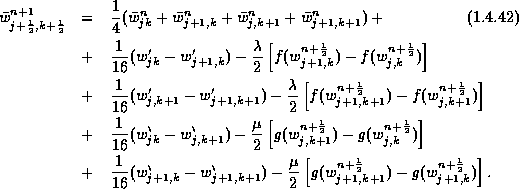
In summary, we end up with a simple two-step predictor-corrector scheme which could be conveniently expressed in terms on the one-dimensional staggered averaging notations

Our scheme consists of a predictor step

followed by the corrector step

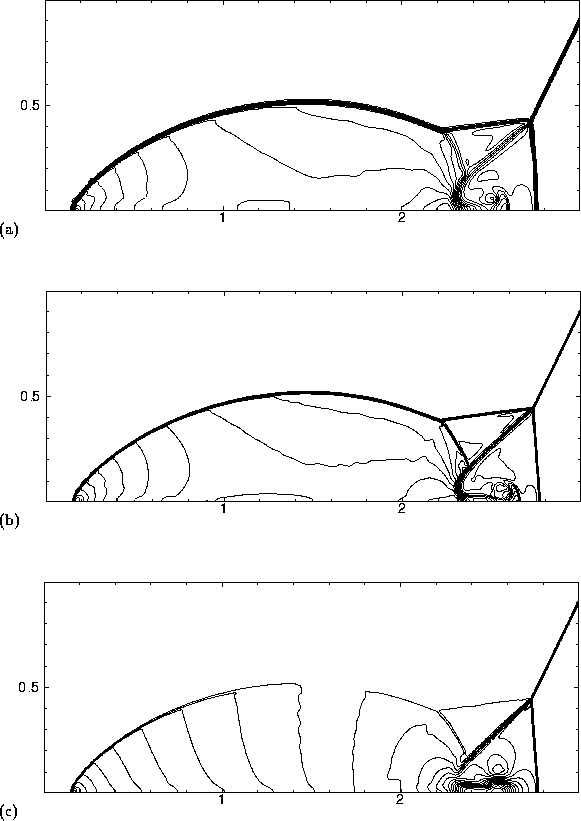
In figures 1.4.8 taken from [16], we present the two-dimensional computation of a double-Mach reflection problem; in figure 1.4.9 we quote from [45] the two-dimensional computation of MHD solution of Kelvin-Helmholtz instability due to shear flow. The computations are based on our second-order central scheme. It is remarkable that such a simple 'two-lines' algorithm, with no characteristic decompositions and no dimensional splitting, approximates the rather complicated double Mach reflection problem with such high resolution. Couple of remarks are in order.

• The two-dimensional computation is more sensitive to the type of limiter than in the one-dimensional framework [31]. In the context of the double Mach reflection problem, the (consult (1.3.16) with ) seems to yield the sharper results.

  
Figure 1.4.8: Double Mach reflection problem computed with the central scheme using limiter with CFL=0.475 at t=0.2 (a) density computed with cells (b) density computed with cells (c) x-velocity computed with cells

 

• No effort was made to optimize the boundary treatment. The staggered stencils require a different treatment for even-odd cells intersecting with the boundaries. A more careful treatment following [26] is presented in §1.4.1. The lack of boundary resolution could be observed at the bottom of the two Mach stems.

We conclude this section with brief remarks on further results related to central schemes. Remarks.

1. Simplicity.

   Again, we would like to highlight the simplicity of the central schemes, which is particularly evident in the multidimensional setup: no characteristic information is required - in fact, even the exact Jacobians of the fluxes are not required; also, since no (approximate) Riemann solvers are involved, the central schemes require no dimensional splitting; as an example we refer to the approximation of the incompressible equations by central schemes, §1.5; the results in [7] provide another example of a weakly hyperbolic multidimensional system which could be efficiently solved in term of central schemes, by avoiding dimensional splitting.

2. Non-staggering. We refer to [15] for a non-staggered version of the central schemes.
3. Stability.

   The following maximum principle holds for the nonoscillatory scalar central schemes:

   
    
   

4. Third-order accuracy. Extensions to third-order accuracy in two space dimensions can be found in [24].

 
• Boundary conditions