Following [22] our goal is introduce a second-order central difference scheme for incompressible flows, based on velocity variables. The use of the velocity formulation yields a more versatile algorithm. The advantage of our proposed central scheme in its velocity formulation is two-fold: generalization to the three dimensional case is straightforward, and the treatment of boundary conditions associated with general geometries becomes simpler. The result is a simple fast high-resolution method, whose accuracy is comparable to that of an upwind scheme. In addition, numerical experiments show the new scheme to be immune to some of the well-known deleterious consequences of under-resolution.
We consider a two-dimensional incompressible flow field, ![]() , so that
, so that
![]() . The equations of
motion for a Newtonian fluid in conservation form are
. The equations of
motion for a Newtonian fluid in conservation form are
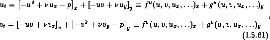
where p is the pressure, ![]() is the kinematic viscosity, and
subscripts denote partial derivatives.
The functions
is the kinematic viscosity, and
subscripts denote partial derivatives.
The functions ![]() and
and ![]() are components of the fluxes of the conserved quantities
u and v.
are components of the fluxes of the conserved quantities
u and v.
The computational grid consists of rectangular cells of sizes
![]() and
and
![]() ; at time level
; at time level
![]() , these cells,
, these cells, ![]() ,
are centered at
,
are centered at ![]() .
Starting with the corresponding cell averages,
.
Starting with the corresponding cell averages,
![]() , we first
reconstruct a piecewise linear polynomial approximation
which recovers the point values
of the velocity field,
, we first
reconstruct a piecewise linear polynomial approximation
which recovers the point values
of the velocity field, ![]() .
For second-order accuracy, the piecewise linear reconstructed
velocities take the form,
.
For second-order accuracy, the piecewise linear reconstructed
velocities take the form,
![]()
As before, exact averaging over a staggered control volume yields
and a similar averaging applies for ![]() .
.
An exact computation yields
![]()
The incompressible fluxes, e.g., ![]() ,
are approximated in terms of the midpoint rule , which in turn
employs predicted midvalues which are obtained from half-step Taylor
expansion. Thus our scheme starts with a predictor step of the form
,
are approximated in terms of the midpoint rule , which in turn
employs predicted midvalues which are obtained from half-step Taylor
expansion. Thus our scheme starts with a predictor step of the form
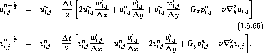
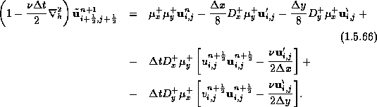
Note that the predictor step is nothing but a forward Euler scheme; conservation form is not essential for the spatial discretization at this stage.
This is followed by a corrector step
Note that the viscous terms are handled here by the implicit Crank-Nicholson discretization which is favored due to its preferable stability properties. Here, we ignore the pressure terms; instead, the contribution of the pressure will be integrated by enforcing zero-divergence fluxes at the last projection step.
Compute the potential ![]() solving the Poisson equation
solving the Poisson equation

Then, the pressure gradient at ![]() is being updated,
is being updated,
![]()
and finally, it is used to evaluate the divergence-free velocity field,
![]()
![]()
In Figure 1.5.15, we plot vorticity contours for
two shear layer problems studied in [5]:
the inviscid ``thick'' shear layer problem
corresponding to ![]() with
with ![]() ,
and a viscous ``thin'' shear layer problem (with
,
and a viscous ``thin'' shear layer problem (with ![]() ),
corresponding to
),
corresponding to ![]() with
with ![]() .
As in [5], both plots in Figures 1.5.15a and
1.5.15b are recorded at time t=1.2, and are subject to
an initial perturbation
.
As in [5], both plots in Figures 1.5.15a and
1.5.15b are recorded at time t=1.2, and are subject to
an initial perturbation ![]() , with
, with ![]() .
.
Further applications of the central schemes for
more complex incompressible flows (with 'variable' axisymmetric
coefficients, forcing source/viscous terms, ...), can be found in
[20],[21].
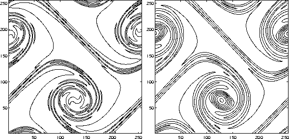
Figure 1.5.15: Contour lines of the vorticity, ![]() ,
at t=1.2 with initial
,
at t=1.2 with initial ![]() ,
using a
,
using a ![]() grid. (a) A ``thick'' shear layer with
grid. (a) A ``thick'' shear layer with
![]() , and
, and ![]() . The contour levels range from -36 to 36
(cf. Figure 3c in Ref. [5]).
(b) A ``thin'' shear layer with
. The contour levels range from -36 to 36
(cf. Figure 3c in Ref. [5]).
(b) A ``thin'' shear layer with ![]() , and
, and ![]() .
The contour levels range from -70 to 70
(cf. Figure 9b in Ref. [5]).
.
The contour levels range from -70 to 70
(cf. Figure 9b in Ref. [5]).