The vorticity formulation

We are concerned with the approximate solution of the 2D Euler (- and respectively - NS) equations, expressed in terms of the vorticity, ,

 
Here, , is the two-component divergence-free velocity field,

 
Equation (1.5.48) can be viewed as a nonlinear (viscous) conservation law,
 
with a global flux, . At the same time, the incompressibility (1.5.49) enables us to rewrite (1.5.48) in the equivalent convective form
 
Equation (1.5.51) guarantees that the vorticity, , propagates with finite speed, at least for uniformly bounded velocity field, . This duality between the conservative and convective forms of the equations plays an essential role in our discussion.

To approximate (1.5.48) by a second-order central scheme (following [16, 31]) we introduce a piecewise-linear polynomial MUSCL approximate solution, , at the discrete time levels, ,
 
with pieces supported in the cells, .

As before, we use the exact staggered averages at , followed by the midpoint rule to approximate the corresponding flux. For example, the averaged flux, is approximated by Analogous expressions hold for the remaining fluxes. Note that finite speed of propagation (of - which is due to the discrete incompressibility relation (1.5.56) below), guarantees that these values are 'secured' inside a region of local smoothness of the flow. The missing midvalues, , are predicted using a first-order Taylor expansion (where and , are the usual fixed mesh-ratios),
 
Equipped with these midvalues, we are now able to use the approximate fluxes which yield a second-order corrector step outlined in (1.5.58) below. Finally, we have to recover the velocity field from the computed values of vorticity. We end up with the following algorithm.

1. Reconstruct
   1. An exact discrete divergence-free reconstruction of the velocity field. We define the discrete vorticity at the mid-cells as the average of the four corners of each cell, i.e.
       
      We then use a streamfunction, , such that , which is obtained in the min-cells, e.g., by solving the five-points Laplacian, . Then, its gradient, recovers the velocity field
       
      Here, and denote averaging in the x-direction and in the y-direction, respectively, such that, e.g.,
      
      Observe that with this integer indexed velocity field, we retain a discrete incompressibility relation, centered around ,
       
      which is essential for the maximum principle in (1.5.1).
2. Predict
   1. Prepare the pointvalues of the divergence-free velocity field , , from the reconstructed vorticity pointvalues, . To this end, use the Biot-Savart solver (1.5.55);
   2. Predict the midvalues of the vorticity, ,
       
      Note: Observe that here we use the predictor step (1.5.53) in its convective formulation (1.5.51), that is, .

3. Correct
   
   1. As in step (2a), use the previously calculated values of the vorticity to compute the divergence-free pointvalues of the velocity, at time , .
   2. Finally, the previously calculated pointvalues of the velocities and vorticity are plugged into the second-order corrector step in order to compute the staggered cell-averages of the vorticity at time ,

      
       
      

The specific recovery of the velocity field outlined above, retains the dual convective-conservative form of the vorticity variable, which in turn leads to the maximum principle [25].

 

As in the compressible case - compare (1.4.43), the main idea in [25] is to rewrite as a convex combination of the cell averages at ,
.

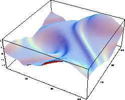
In figure 1.5.14 we show the central computation of a 'thin' shear-layer problem, [5]. For details, consult [25].

 
Figure 1.5.13: t = 8 , 64*64

\

 
Figure 1.5.14: t = 8 , 128*128  

The ``thin'' shear-layer problem, solved by the second-order central scheme
(1.5.53),(1.5.58) with spectral reconstruction of the velocity field.